Assignment tests (Go to assignment test web calculator [old, unmaintained version])
The idea behind assignment tests is to use individual genotypes to assign individuals to populations or clusters. Paetkau et al. (1995) developed the first assignment test approach for use on bears. The idea was fairly simple. Given a set of populations, and the allele frequencies of those populations, what is the likelihood of a given individual�s genotype in the population in which it was sampled versus its likelihood in the other populations in the set? An individual is assigned to the population for which it has the highest likelihood.
Let�s take a simple example with four alleles at one locus (a, b, c, and d) and three alleles at a second locus (k, l, and m):
|
|
a |
b |
c |
d |
k |
l |
m |
|
Pop1 |
0.2 |
0.1 |
0.3 |
0.4 |
0.5 |
0.3 |
0.2 |
|
Pop2 |
0.5 |
0.3 |
0.1 |
0.1 |
0.1 |
0.6 |
0.3 |
Now, say we have an individual with the genotype abll. Its probability in Pop 1 is (2*0.2*0.1)*0.32 = 0.0036. Its probability in Pop 2 is (2*0.5*0.3)*0.62 = 0.108. The likelihood in Pop 2 is considerably higher than the likelihood in Pop 1. We �assign� it to Pop 2. Conversely, an individual with the genotype cdkl would be much more likely in Pop 1 (0.072) than in Pop 2 (0.0024). [We need to calculate heterozygote probabilities as 2 times the product of the gene frequencies; remember the Punnett square idea that it could get A from Dad and a from Mom OR a from Dad and A from Mom ]. With a large number of loci, and the presence of rare alleles, we use logarithms to make the numbers easier to assess.
Fig. 1. Assignment graph for individuals sampled in two populations. Individuals in red were sampled in Pop 1, those in blue in Pop 2. Above the line are individuals �assigned� to Pop 2, below the line individuals assigned to Pop 1. Note that, for this example, one Pop1 individual is assigned to Pop 2, and one Pop 2 individual is assigned to Pop 1. Such �misassigned� individuals might represent immigrants from the other population, or the descendants of such immigrants (or it could occur on the wrong side of the line by chance; the further from the line, the less likely the deviation occurs by chance; the more highly polymorphic loci we have, the stronger the evidence).
The problem of zeros. If an allele does not occur in a population (px = 0) then the assignment probability of an individual to that population will be 0. Several methods (described on the now-unsupported assignment calculator web site http://www2.biology.ualberta.ca/jbrzusto/Doh.php) exist for adjusting the allele frequencies in the event of zeros.
Several alternatives now exist for assignment tests. One of these is to use Bayesian methods for deciding on the likelihood of assignment. J.-M. Cornuet has a package of such approaches at his web site
http://www.montpellier.inra.fr/URLB/geneclass/geneclass.html
The program runs in Windows, and has a range of options for dealing with the zero problem.
A variant on the assignment approach is to allow the data themselves to determine the population has subpopulations and, if so, how many. The program Structure uses Hardy-Weinberg equilibrium (HWE) assumptions to create clusters. That is, it sequentially assesses the fit of portions of the data to a set of k clusters, with each cluster maximally obeying HWE structure. Because an algorithm/equation underlies the expectation, maximum likelihood estimation (MLE) is suitable for the decisions about the k clusters.
The program Structurama by Huelsenbeck (http://www.structurama.org/), also calculates the algorithms of Pritchard (2000) with a few extra twists.
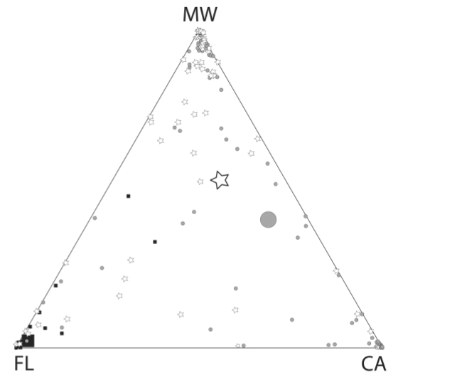
Fig. 2. Assignment graphic for a three
cluster (k = 3) assessment of Burrowing
Owl populations, using the program Structure. Each
of the three vertices represents exclusive assignment to one of the three
clusters; points more toward the center have affinities with all three
clusters. The square symbols are
Florida owls (note that their centroid is very close to the Florida vertex), the
triangles are CA populations (centroid basically right in the middle of the line between CA and MW, meaning we really can't tell much about owls sampled in California -- they could just as well belong to the MW cluster) and the stars are Rocky Mt. region individuals. Many of the California and Rocky Mt.
region individuals were �misassigned�.
References:
Paetkau, D, W. Calvert, I. Stirling, and C. Strobeck. 1995. Microsatellite analysis of population structure in Canadian polar bears. Mol. Ecol. 4: 347-354.
Pritchard, J.K., M. Stephens, and P. Donnelly. 2000. Inference of population structure using multilocus genotype data. Genetics 155: 945-959.