Lecture 3.
Population Genetics I.
Introduction to Population Genetics
Return
to index page
Required readings: Avise text, pp. 248-257,
Gillespie book Chapters 1, 2 and 5.
Population genetics is the study of Mendel�s laws,
the Hardy-Weinberg principle and other genetic principles as they apply
to entire populations of organisms. Population genetics describes genetic
variation in populations, and determines, by observation, experiment and theory, how that variation changes over time and space.
In other words, how much variation exists in natural populations, and how can we explain
variation in terms of origin, maintenance, and evolutionary importance?
What�s useful about population genetics?
-
Management issues. We can answer questions
about patterns and trends in genetic variability, gene flow (are populations
genetically connected?), patterns of dispersal (do males or females tend
to disperse further?), Ne (effective population size,
which we will address below), fluctuations in population size (called "bottlenecks"
and also addressed below), forensics applications (legal cases -- does
the carcass in the suspect�s freezer match the poached animal found by
a warden), and population size estimation (using genetic mark-recapture
techniques).
-
Conservation of threatened and endangered species.
Assessment
of genetic variability to prevent inbreeding depression (useful only for captive breeding programs aimed at highly valued, charismatic organisms such as black-footed ferrets), recognition
of threatened and endangered species (is this candidate "species" actually
distinct from a more widespread common form found elsewhere?), and molecular
forensics for law enforcement (is this animal part from an endangered ferret
or a legal mink?).
-
Evolutionary understanding. Population
genetics provides a coherent framework for understanding how biodiversity
is created and maintained. Population genetics helps explain the spread of traits under the influence of natural selection (a huge topic, which I will largely ignore).
Hardy-Weinberg Principle
The Hardy-Weinberg principle (and its predicted equilibrium) is the
cornerstone of population genetics. Developed independently by George Hardy and
Wilhelm Weinberg in the early 1900�s, the Hardy-Weinberg principle is a
model that relates allele frequencies to genotype frequencies. Like most
models, Hardy-Weinberg is a simplification of real world complexities
-- but it has amazing explanatory power nonetheless.
Remember (memorize) the five major assumptions
that lead to a Hardy-Weinberg equilibrium (click links to see discussion of each force):
{Three additional assumptions are that the organisms are diploid, reproduce
sexually and have non-overlapping generations}.
Violations of any of the five major assumptions are the
primary forces that drive evolutionary change.
Remember that an allele is a variant form of a gene (piece of
DNA) at a single locus (Latin for "place", so we are referring to a particular
stretch -- for example a stretch of 275 base pairs on Chromosome 13).
An allele frequency (geneticists call it "gene frequency") is therefore
a measure of the commonness of an allele in a population (the proportion
of a specific allele in a population -- how common is the A ["big
A"] allele, or the a ["little a"] allele). A genotype is
the specific allele composition for a certain locus or set of loci (Aa,
AA,
or AaBBcc for several loci vs. a second genotype AabbCc).
Genotype frequency is a measure of the commonness of a genotype in a population;
i.e., the proportion of a specific genotype in a population. Two major
terms are important in discussing genotypes: homozygote and heterozygote.
A homozygote has two copies of the same allele (e.g., AA or bb).
A heterozygote has two different alleles at a given locus (e.g., Aa
or Dd). Because the allele and genotype frequencies are proportions
they always sum to 1.0, if we have included all the possible variants.
Allele frequencies:
p + q = 1
Eqn 3.1
Expected genotype frequencies:
p2 + 2pq + q2
= 1
Eqn 3.2
The possible range for an allele frequency or genotype frequency therefore
lies between zero and one, with zero meaning complete absence of that allele
or genotype from the population (no individual in the population carries
that allele or genotype); a one means complete fixation
of the allele or genotype (fixation means that every individual in the
population is homozygous for the allele -- i.e., has the same genotype
at that locus).
With the five assumptions given above, one can
calculate the genotype frequencies for a gene with two alleles (A
and a). The frequency of homozygous genotype AA is the probability
of one allele A being in combination with another allele A.
The expected frequency is simply the product of the separate allele frequencies.
We will use the term p to refer to the frequency of allele A:
Frequency of AA = p2
Eqn 3.3
The frequency of heterozygous genotype Aa is the probability of
allele A being in combination with allele a. Note that there
are two possible ways to get those combinations -- A from Dad and
a
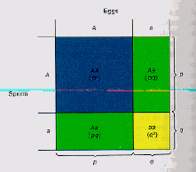
from Mom, or vice versa (examine Fig. 3.1 below).
Frequency of Aa = 2pq
Eqn 3.4
The frequency of homozygous genotype aa is the probability of one
allele a in combination with another allele a.
Frequency of aa = q2
Eqn 3.5

Fig. 3.1. Diagram of Hardy-Weinberg genotype
proportions. Given a locus with two alleles designated A and a
that occur with frequencies p and
q, the chart shows the
genotype frequencies (p2, 2pq, and q2)
as differently colored areas. Note that the heterozygotes (blue + yellow
= green) can be formed in two different ways (in terms of combination theory,
this means order is not important). Extending this logic and its implications to multiple alleles and multiple loci provides the basis for much of the core theory of population genetics.
Example: if p = 0.75 and q = 0.25 we can use Eqns 3.3, 3.4,
and 3.5 to calculate the expected genotype frequencies.
AA = p2 = 0.75 * 0.75
= 0.5625
Aa = 2pq = 2 * 0.75 * 0.25 =
0.375
aa = q2 = 0.25 * .025
= 0.0625
Eqns 3.6
The values we have just calculated are EXPECTED genotype frequencies
IF
the Hardy-Weinberg assumptions hold. We now turn to how we could check
that from actual OBSERVED genotypic data (such as the microsatellite data
for Wyoming black bears). In order to calculate allele frequencies all
we need are the observed genotype frequencies. [No assumptions needed about the five forces, but what statistical requirement.assumption do we need to have in place?]
p = p2 + (2pq/2) and q = q2
+ (2pq/2)
Eqn 3.7
Let's look at an example from the beginning. We will examine a population
of trout with a di-repeat microsatellite marker that has two alleles, 120
and 122. For simplicity, let�s call allele 120 A and allele 122
a.
We genotype 100 individuals and find genotype frequencies of
AA
= 0.25, Aa = 0.5, and aa = 0.25 (check that when summed these
genotype frequencies add to one). We ask the question of whether this population
is in Hardy-Weinberg equilibrium. We first need to calculate the p
and q (allele frequencies of A and a; note that the
A
and a are names for the alleles themselves, the p and
q refer
to the frequencies of those alleles). We calculate the frequencies
using Eqns 3.6.
p = p2 + (2pq/2) = 0.25 + (0.5/2)
= 0.5
q = q2 + (2pq/2) = 0.25 + (0.5/2)
= 0.5
Eqns 3.8
We see that the allele frequencies sum to one, as required by Eqn 3.1.
Using the allele frequencies, we then calculate the expected genotype frequencies
using Eqns 3.3, 3.4, and 3.5.
AA = p2 = 0.5 * 0.5 = 0.25
Aa = 2pq = 2 * 0.5 * 0.5 = 0.5
Aa = q2 = 0.5 * .05 = 0.25
Eqns 3.9
The expected genotype frequencies are same as the observed genotype frequencies
(from the microsatellite data). This tells us that our population is
in Hardy-Weinberg equilibrium. If the expected genotype frequencies calculated
from the allele frequencies were not the same as the observed genotype
frequencies our population would not be in Hardy-Weinberg equilibrium --
we assess whether the difference is statistically significant using
a chi-square test, as we will see shortly. [Note that statistical significance is not a guarantee of biological significance].
The expected frequency distribution of genotypes AA, Aa,
and aa in proportions p2, 2pq and q2
respectively is called the Hardy-Weinberg equilibrium. If the population
meets the eight assumptions listed above, then
the population will go to the Hardy-Weinberg equilibrium in the first generation,
and remain there. Again, the Hardy-Weinberg principle and its predicted
equilibrium, is a simple model that serves as a starting point for examining
the genetic structure of populations.
Violating Hardy-Weinberg assumptions
How likely are we to meet the major assumptions
of random mating, no drift, no mutation, no migration, and no natural selection?
If we violate the assumptions, how much difference does it make? Here is
a list of processes that violate the Hardy-Weinberg assumptions and some
discussion of each of them. These "big five" forces are the major engines of evolutionary change. An important point is whether the given force tends to increase or decrease the genetic variability in populations.
• Non-random mating (tends to reduce genetic variation)
Random mating means that alleles (as carried by the
gametes -- eggs or sperm) come together strictly in proportion to their
frequencies in the population as a whole. Example: if p = 0.6 and
q
= 0.4, then the probability of an Aa heterozygote is 0.48 (the product
of the allele frequencies, plus consideration of the fact that two ways
exist to make a heterozygote; see Fig. 3.1). Situations
where the random mating assumption does not hold include:
-
Inbreeding � cases where relatives (e.g., siblings, cousins) have
a greater probability of mating with each other than with other members
of the population.
Inbreeding will tend to decrease heterozygosity without affecting allele
frequencies.
-
Geographic structuring � in many cases individuals are more likely
to mate with geographically proximate individuals than with more distant
individuals.
Geographic structuring is essentially an extended form of inbreeding.
-
Positive/Negative Assortative mating � in positive assortative mating
(usually called just assortative mating) individuals of a given phenotype
or genotype tend to mate with similar individuals (e.g., A1A1
tend to mate with other
A1A1).
Assortative mating will decrease heterozygosity (put like alleles together)
without affecting gene frequencies.
In negative assortative mating (usually called disassortative mating)
individuals tend to mate with dissimilar individuals.
Disassortative mating will tend to increase heterozygosity (put unlike
alleles together) without affecting gene frequencies.
-
Rare allele advantage. In some mating systems a male bearing
a rare allele will have a mating advantage.
Rare allele advantage will tend to increase the frequency of the rare
allele and hence increase heterozygosity.
-
Mating system effects � in a polygynous mating system one or a few
males that obtain a disproportionate share of the matings will be over-represented
genetically (this differs from the rare allele effect mainly in that the
male's success is not dependent on having rare alleles -- any rare alleles
he does happen to have, however, will increase in frequency in the next
generation). Variance in mating success can change both gene frequencies
and the level of heterozygosity (up or down will depend on the genotypes
of the successful males relative to the frequencies in the population).
Often, the impact of a moderate amount of non-random mating has a negligible
impact on our conclusions about the patterns and causes of genetic variation.
• Random genetic drift (always reduces genetic variation)
The effect of random genetic drift is inversely proportional to population
size. Allele frequencies change because the genes appearing in
offspring are not a perfectly representative sampling of the parental genes
(in a finite population). Since drift is a random process, outcomes of
drift must be stated as probabilities. Drift removes genetic variation
from the population at a rate inversely proportional to population size.
As population size decreases the force of drift increases, and vice versa.
Drift also affects the probability of survival of new mutations. The probability
that an allele will move to fixation is equal to
its frequency in the population -- an allele with a frequency of 0.2 (20%)
has a 20% chance of fixation. New alleles introduced by mutation almost
inevitably begin at low frequencies and have a low probability of fixation.
Drift can lead to the loss of rare alleles and the fixation of common alleles.
If the population is large, however, drift has little effect.
Marble analogy: Think of a jar containing a million marbles
in ten different colors. If we draw a random sample of 500,000 it
will almost certainly contain all the marbles in proportions very similar
to the original proportions. If we pick only five marbles, however, we
will definitely have a biased sample (we can�t have picked more than 5
of the 10 alleles -- any duplicates and we'll have even fewer alleles).
Even if we take a sample of 50, we will be unlikely to maintain the proportions
of the original million -- the small sample prevents us from drawing a
representative array. Similarly, drift is inversely proportional
to population size -- large population = minor drift, small population = major drift.
Drift can have major effects on endangered (small, almost by definition)
populations. For other species it can take a long time (thousands, hundreds
of thousands or even millions of years) for drift to have large effects.

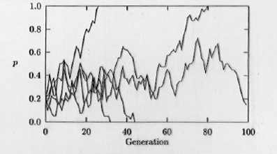
Fig. 3.2. Computer simulation of genetic
drift. The fate of the A1 allele (with frequency p,
on
the Y-axis) is shown in five replicate populations for a time course
of 100 generations (time on the X-axis). Note that if
p drops
to 0 or rises to1.0 then A1 will be lost (0) or reach
fixation (1.0). Those frequencies (0 and 1.0) are therefore called "absorbing
boundaries". Notice also the jagged trajectories that often characterize
random processes.
• Selection (reduces genetic variation)
Selection is the differential survival and reproduction of phenotypes
that are better suited to the environment or to obtaining mating success.
Selection is the evolutionary force responsible for adaptation to
the environment. Selection generally removes genetic variation from the
population (occasionally special circumstance such as "frequency-dependent"
or "balancing" selection can serve as forces maintaining variation). Alleles
that confer advantages in survival or reproduction will tend to be represented
in greater proportion in the next generation. After numerous generations
(the time required will depend on the intensity of selection and the heritability
of the trait), the advantageous allele will tend to spread to fixation. It is sometimes useful (and almost always interesting) to distinguish, as Darwin did, between natural and sexual selection.
If drift and natural selection tend to reduce genetic variation, what
maintains or increases it? -- Mutation.
• Mutation (increases genetic variation and introduces novel variants)
Mutation is the process that produces a gene or chromosome set differing
from the wild-type (ancestral allele). Mutation restores genetic variation
to a population by producing novel alleles. Mutation is difficult to measure
or observe directly, and rates of mutation can vary between loci. It is
usually a weak force and therefore tends not to pull populations very far
from Hardy-Weinberg equilibrium -- over long enough time periods,
though, even a weak force can have major effects (e.g., the erosion of
the Grand Canyon). Much of the neutral theory of genetic variation
is based on a calculation of the balance between drift and mutation as
forces of change.
• Genetic Migration (distributes and homogenizes genetic variation)
Genetic migration is the permanent movement of genes from one population
into another. Migration can restore genetic variation into isolated and
differentiated populations or reduce variation among populations when it
occurs frequently. Assessing the patterns and importance of genetic migration
(often referred to as "gene flow") is one of the major aims of population
genetics. [Note that this definition of migration is very different from that for the seasonal back and forth movement of birds, for example, from breeding grounds in the temperate zone to non-breeding grounds in the tropics. Migration, in that sense may have little effect on permanent movement of alleles].
Some absolute basics about probability and combination
theory:
Much of population genetics involves manipulations of equations that
have a base in either probability theory or combination theory. We
saw combination theory in action when we used the formula for the number
of distinct unrooted trees as a function of the number of OTUs. The
basic Hardy-Weinberg equation p2 + 2 pq + q2
is a probabilistic one (with the addition that since order is unimportant
we account for two ways to get heterozygotes).
Rule 1: If you account for all possible events, the probabilities
sum to 1. [e.g., p + q = 1 for a two-allele system].
Rule 2: The probability that two independent events occur is
the product of their individual probabilities.
[e.g., probability of a
homozygote is q*q = q2].
Punch line: Genetic techniques examine individual variation to
discern the emergent properties of populations and higher taxa. We can examine genetic
variation at multiple scales -- from the level of the individual
(e.g., forensics applications) to analysis of higher taxa in systematic
and taxonomic studies. Population genetics integrates a broad spectrum of process
and pattern -- geneticists simplify by including only essential forces in their models and by making simplifying assumptions that, if violated, do not change
the qualitative conclusions. A traditional first step is to build from the
Hardy-Weinberg principle -- despite its admittedly unrealistic assumptions
of random mating, no drift, no mutation, no migration, and no natural selection.
In situations where one or more of these assumptions is clearly violated
in a major way, a variety of more complex models can then be brought to
bear on the problem.
Return to top of page

