Lecture 35 (21-Apr-06)

Return to Main Index page       Go back to notes for Lecture 34,  19-Apr    Go forward to lecture 36  24-Apr-06

Go to worked example for take-home exam

Population Genetics (continued)

      Go to Glossary of genetic terms

       Go to worked F_ST calculation web page.

Violating Hardy-Weinberg assumptions (continued)

I ended the last lecture with a discussion of how non-random mating can produce genetic and evolutionary change.  We will now examine each of the other four forces of evolutionary change -- migration, mutation, drift and selection.

Genetic Migration (high gene flow maintains similarity among populations)

Genetic migration is the permanent movement of genes from one population into another. Migration can restore genetic variation into isolated and differentiated populations or reduce variation among populations when it occurs frequently. Assessing the patterns and importance of genetic migration (often referred to as "gene flow") is one of the major aims of population genetics.  High gene flow will tend to maintain genetic similarity among  populations.   For example, new alleles arising by mutation in one population, will be carried to other populations by dispersing individuals.

Mutation (random source of new genetic variation)

Mutation is the random process that produces a gene or chromosome set differing from the wild-type (ancestral allele). Mutation restores genetic variation to a population by producing novel alleles. Mutation is difficult to measure or observe directly, and rates of mutation can vary between loci. It is usually a weak force and therefore tends not to pull populations very far from Hardy-Weinberg equilibrium  -- over long enough time periods, though, even a weak force can have major effects (e.g., the erosion of the Grand Canyon).  When populations are separated by geographic barriers, they will tend to develop independent mutations and if enough different mutations occur, the populations will diverge enough to become distinct species.

Drift (a random genetic sampling process that can change allele frequencies and lead to fixation or loss of alleles)

Now we will turn to another random force -- genetic drift.  Although it has a negligible effect in very large populations,  genetic drift can be a major force in changing gene frequencies in small populations.  Random genetic drift is a change in allele frequencies that occurs because the genes appearing in offspring are not a perfectly representative sampling of the parental genes. Since drift is a random process, outcomes of drift must be stated as probabilities. Drift removes genetic variation from the population at a rate inversely proportional to population size. As population size decreases, the force of drift increases, and vice versa. Drift also affects the probability of survival of new mutations. The probability that an allele will move to fixation is equal to its frequency in the population -- an allele with a frequency of 0.2 (20%) has a 20% chance of fixation. New alleles introduced by mutation almost inevitably begin at low frequencies and have a low probability of fixation. Drift can lead to the loss of rare alleles and the fixation of common alleles. If the population is large, however, drift has little effect. Think of a jar containing a million marbles in ten different colors. If we draw a random sample of a million (with replacement) it will almost certainly contain all the marbles in proportions very similar to the original proportions. If we have only 20 marbles, however, and pick a sample of 20 with replacement, we are quite mlikely to have some of the 10 colors missing, and some colors overrepresented. Even if we sample with replacement from a population of 100, we will be unlikely to maintain the proportions of the original population -- similarly, drift is inversely proportional to population size -- large population, minor drift, small population, major drift. Drift can have major effects on endangered (small almost by definition) species. For other species it can take a long time (thousands, hundreds of thousands or even millions of years) for drift to have large effects.

Fig. 35.1. Computer simulation of genetic drift acting within a small population (20 individuals). The fate of the A allele (with starting frequencies of p = 0.2, on the Y-axis) is shown in five replicate populations of 20 individuals, for a time course of 100 generations (time on the X-axis). Note that if p drops to 0 or rises to 1.0 then A will be lost (0) or reach fixation (1.0). [Fixation means that all the individuals in a population have that allele  -- i.e., no genetic variability exists at that locus in that population]. Those frequencies (0 and 1.0) are therefore called "absorbing boundaries".  Once the frequencies hit either boundary they won't change (unless mutation adds another allele or "recreates" the lost allele).  Notice also the jagged trajectories that often characterize random processes.

Selection is the differential survival and reproduction of phenotypes that are better suited to the environment or to obtaining mating success. Selection is the evolutionary force responsible for adaptation to the environment.  Selection generally removes genetic variation from the population (occasionally special circumstance such as "frequency-dependent" or "balancing" selection can serve as forces maintaining variation). Alleles that confer advantages in survival or reproduction will tend to be represented in greater proportion in the next generation. After numerous generations (the time required will depend on the intensity of selection and the heritability of the trait), the advantageous allele will tend to spread to fixation.

How the forces combine: Dodo as case history

Non-random mating, drift and selection tend to reduce genetic variation.  What maintains it? -- Mutation.  For neutral genetic markers (not subject to selection) we will often be interested in the balance between drift and mutation, and the level of gene flow that prevents differentiation among populations.  Small isolated populations will tend to have no gene flow to connect them to related populations elsewhere.  Their mutations will increase or maintain genetic variation but  those mutations will be different from the mutations arising in the related populations.  Finally, the effects of drift will tend to randomly fix some alleles and cause the loss of other alleles.  The result can be fairly rapid evolution of very different forms -- the Dodo (familiar to many from Alice in Wonderland) was a very peculiar-looking flightless bird found on the island of Mauritius (way off the island of Madagascar and highly isolated out there in the Indian Ocean).  The Dodo was driven to extinction by overharvest and the introduction of domestic animals in the late 17th century.  Recent genetic analyses confirm an earlier suspicion that the Dodo was an extremely divergent form of pigeon.  Drift, selection, mutation and low gene flow all combined to cause it to become something that few would recognize as a relative of the familiar Rock Dove (city pigeon) or Mourning Dove.
 

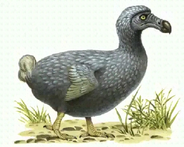
Fig. 35.2.  Artist's reconstruction of the Dodo, a large (> turkey-sized), flightless bird of Mauritius (Indian Ocean), driven to extinction in the late 17th century.  Genetic analyses of dried tissue from the one (partial) specimen in the British Museum indicate that the Dodo is a type of pigeon.  Mutations, low gene flow, natural selection, genetic drift and probably non-random mating likely all combined to cause the extreme divergence that separates this unusual  bird from its closest mainland relatives.  Other, usually slightly less dramatic, examples abound of the divergence of island populations from their mainland progenitors.  In the Rocky Mountain west mountain chains may act as "islands" of habitat, creating the conditions for genetic divergence among populations on different mountain chains.

Measuring genetic variation in natural populations -- Heterozygosity (or gene diversity)

When we actually go out to assess genetic variability in natural populations, some of the first and most important measures we take are the observed and expected heterozygosities.  These tell us how much variation exists in the population and how that variation is distributed across the alleles in the loci we are examining.

Heterozygosity is of major interest to students of genetic variation in natural populations. It is often one of the first "parameters" that one presents in a data set.  It can tell us a great deal about the structure and even history of a population. Just for example, very low heterozygosities for allozyme loci in cheetahs and black-footed ferrets indicate severe effects of small population sizes (population bottlenecks or metapopulation dynamics that severely reduced the level of genetic variation relative to that expected or found in comparable mammals).

Several measures of heterozygosity exist. We will focus primarily on expected heterozygosity (H_E, also written as H_exp and termed  gene diversity by population geneticist Bruce Weir). The simplest way to calculate it for a single locus is as:

                                                                                                Eqn 35.1

                                                                                Eqn 35.2

Expected heterozygosity is equal to one minus the expected homozygosity.

Why does it work to take the sum of the squared gene frequencies and subtract that from one? Let's think back to basic Hardy-Weinberg:

p² + 2 pq + q² = 1

6 + 5 + 4 + 3 + 2 + 1 = 21 = [6*(6+1)]/2      or more generally

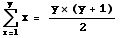                                   Eqn 35.3

                           Eqn 35.4

Heterozygosity is maximal when the allele frequencies are equal.  What does heterozygosity tell us and what patterns emerge as we go to multi-allelic systems? Let's take an example. Say p = q = 0.5. The expected heterozygosity, H_exp, for a two-allele system is described by a concave down parabola that starts at zero (when p = 0) goes to a maximum at p = 0.5 and goes back to zero when p = 1.

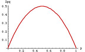
Fig. 35.3. Expected heterozygosity (H_exp = 2pq) for a 2-allele system as a function of allele frequency, p.  Note that the heterozygosity peaks at a value of 0.5, when the allele frequencies are equal (p=q).  It is minimal at both extremes -- in those cases everyone is a homozygote of one type or the other.

p₁ = p₂ = p₃ = ….p_k

Individual’s-eye view of heterozygosity (H_exp = probability that an individual will be heterozygous)

Here is a way that I like to think of heterozygosity (H_exp ). It is the (expected) probability that an individual will be heterozygous at a given locus (or over the assayed loci for a multi-locus system). For many human microsatellite loci, for example, H_exp is often > 0.85, meaning that you have a > 85% chance of being a heterozygote.

From heterozygosity to F-statistics: a way of assessing genetic differences among populations.

Heterozygosity is one of the best ways to approach the analysis of differences among populations.  We will use heterozygosities as the basis for calculating something called F-statistics. F-statistics are a general statistical tool for analyzing variances (variation in gene frequencies).  They are not restricted to genetic applications.  In the 1930's, however, Sewall Wright of the University of Chicago, pioneered their application to genetic studies of natural populations.  With the rise of genetic laboratory techniques such as allozymes in the '60's and '70's, F-statistics became one of the fundamental tools of population genetics applied to natural populations.

Local (per subpopulation) F, with no subscript (or just one to denote the subpopulation):
    Within a subpopulation, we can calculate the unsubscripted statistic, F, as the ratio of (the difference between expected and observed heterozygosity) to (expected heterozygosity).  The general formula is:

                                                                                          Eqn 35.5

Global (over a set of subpopulations) F-statistics, with two subscripts:
    For a set of subpopulations for which we have genotypic information, we usually consider F-statistics to have three levels, each named by a different set of subscripts.  These reflect three levels of biological organization, Individuals, Subpopulations, and the Total population (a set of >= 2 subpopulations).  We can assess heterozygosities at each of these levels and use them as the building blocks for creating levels of F-statistics.  Here are the three levels.  The first two are the most important:

    F_IS is sometimes called the inbreeding coefficient,  It assesses global variation in Individuals, relative to the variation in their Subpopulation.
            If F_IS is negative, then the set of  subpopulations, as a whole, is outbred (has an excess of heterozygotes).
            If F_IS is positive then the set of  subpopulations, as a whole, is inbred (deficiency of heterozygotes).

    F_ST is probably the most important.  It assesses the variation in the Subpopulations relative to that in the Total population.
            It can have values between 0 and 1.0 (i.e., it cannot be negative).
        F_ST of zero means that all the subpopulations have the same gene frequencies.
        F_ST of 1.0 means that the subpopulations have completely nonoverlapping sets of alleles (the subpopulations are fixed for different alleles).
                     Natural populations tend to have F_ST values that range between near zero up to just greater than 0.5.
                     Values of F_ST above approximately 0.2 are considered "high".

    F_IT is relatively rarely used.  It assesses the variation in Individuals relative to the variation in the Total set of subpopulations.

In general, F-statistics can range from values of -1 to +1.  As we saw above, F_ST has a more restricted ranges of possible values (0 to 1).

To calculate the F-statistics above we use three kinds of heterozygosity values.

        H_I is the average observed heterozygosity in individuals.

        H_S is the expected heterozygosity (gene diversity) of subpopulations, calculated as the weighted average across a set of subpopulations.
                      We use Eqn 35.1 to calculate the expected heterozygosity in each subpopulation, then weigh the results by the subpopulation sizes

        H_T is the expected heterozygosity over the whole set of populations.
                      We use the global gene (allele) frequencies and then plug them in to Eqn 35.2 to calculate it.

I have set up a complete worked example of calculating gene frequencies, observed versus HWE expected genotypic counts, heterozygosities, and F-statistics on a separate web page.  The example is a two-allele, three population case.  You will calculate the same sets of statistics for a three-allele, four-population case in Homework 8.

  Go to worked F_ST calculation web page.

§§§§§§§§§§§§§§§§§§§§§§§§§§§§§§§§§§§§§§§§§§§§§§§§§§§§§§§§§§§§§§§

Return to top of page                           Go forward to lecture 36 , 24-Apr-06