Eqn 15.1
Return to Main Index page Go to Lecture 16 Go to Lecture 17
Go to movie of discrete logistic 2-cycle (r = 2.2) case Go to movie of discrete logistic converge-to-K (r = 1.5) case
Intraspecific competition -- discrete logistic equation
very high (chaotic) r case
Embedded QuickTime Movie (from Mathematica notebook ChaosMovie.nb)
Click on the image below to start the "movie". A control bar will appear below the graph; the various buttons will allow you to stop and start it.
Fig. 1. One-dimensional "map" of the discrete logistic (Eqn 15.1, above) with r = 3 and K = 1,000. Note that the population never settles on any value or set of values. We start with an N(t) value on the X-axis, move up to the "map" (red line) to get an N(t+x) value and then take the corresponding Y-value by going over to the 1:1 black line, then again move to the red line. Tracing the map is therefore a process of going back and forth from the red map line to the black N(t+x) = N(t) 1:1 line (like a box step dance -- "up, right, down, left"). Following the map this way gives us the successive population sizes over time. Note that the trajectory moves away from the unstable equilibrium point (at K = 1,000) and toward a chaotic pattern of highly variable population sizes. Here, the "movie" runs for 99 time steps. We could go for much longer without ever repeating our steps.
The high r value here is what drives the cycle.
Return to top of page
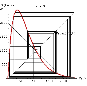
Fig. 2. Static view of the trajectory for 99 time steps in the chaotic range from a starting N0 of 950.
Note that values near unstable equilibrium point K (1,000) will spiral outward. The places where the values spend more time (and develop thicker black lines) are called "strange attractors" in chaos theory.