Lecture 1. Intro. to Genetic Markers. Mon 25-Aug-08

The subject of this course is the use of genetic molecular markers to make inferences about natural populations.

Terms in red italics are (or should be) in the Glossary of terms (link on the Index page).

Kinds of questions and approaches:

The kinds of things we will want to know range from

Individualization: does the elk carcass in the freezer individually match the evidence in the field?
to
Relatedness: can kin selection (high relatedness) explain cooperative courtship display in a tropical bird?
to
Assignment to population source: do bear populations across Wyoming show sufficient differentiation to allow us to assign unknown samples to a source area (with reasonable to high confidence)?
to
Population genetic structure: what forces could explain the observed patterns of genetic differentiation among populations of Species X (bears, jays, species of your choice)?
to
Species boundaries: are these two forms of jay a single species or two distinct species?
to
Phylogenetic trees: where do cetaceans fit in a phylogenetic tree of mammalian groups?
to
what is the grand arrangement of the tree of life in terms of kingdoms and phyla?

That is, we will move across the entire spectrum from individual identification to higher level systematics. Largely because it is the core of my expertise (and because its principles extend easily all the way down to individual ID and often all the way up to phylogenetic inference) the core of the course will be the principles of population genetics.

Why do we want this sort of information? The reasons will range from

legal/forensic (wildlife crimes),
to
answering evolutionary puzzles (how or why does this behavior or mating system occur?),
to
assessing plant, fisheries or wildlife populations for management reasons
to
solving conservation problems — which taxa should we focus on for conservation, where do areas of high endemism occur, what are the consequences of anthropogenic (human-induced) changes?

A quick overview of the major portions of the course. {I don’t expect you to know or digest the details of the examples given in the Tables and Figures below, just to get a feel for the kinds of problems one can tackle}.

Phylogeny and systematics: How are taxa arranged on the tree of life? The study of systematics and taxonomy began with morphological data (bones, muscles) but has been revolutionized by molecular approaches. Both mitochondrial and nuclear DNA have proven very useful for making inferences concerning the relationships of taxa -- ranging from the species level to reorganization of the kingdoms of life. We will begin by actually working some simple algorithms for building phylogenetic trees. We will examine various alternative strategies for tree-building, as well as gaining a little familiarity with some of the software now available for phylogeny construction. We will learn what data we need to gather, the analytical tools available , and the kinds of problems addressed.

Example: How do we use a UPGMA or neighbor-joining technique to go from a matrix of molecular data to a phylogenetic tree hypothesis?

Table 1.1. MtDNA sequence data for great apes: No. of differences (below diagonal) and Jukes-Cantor distances (above diagonal). Data from Weir, 1996

Fig. 1.1. UPGMA tree for great apes from Jukes-Cantor distances from mtDNA data. By using well-established algorithms we can go from lab. molecular data to a table of genetic distances (Table 1) to the phylogram shown here, which shows a branching pattern of relatedness between the taxa. Here we see that humans and chimps form a clade (a monophyletic group), as do humans, chimps and gorillas, etc.

Fig. 1.2. Fitch-Margoliash tree for the great apes from the data in Table 1. The way the tree is drawn (consider the length and orientation of the branches) suggests that some of the assumptions and implications of this tree are different from those of the UPGMA tree in Fig. 1.1.

Population genetics: Next, we will tackle population genetics — the theoretical underpinnings of population genetics and how, in practice, we can apply those principles to problems in evolutionary biology, management and conservation.

Population genetics is the study of genetic polymorphism (DNA variation) and its organization at various levels (how genetic variability is organized within individuals, among individuals, within populations and among populations).

Again, we will work with real data sets to get hands-on experience in data analysis, while reading articles that discuss the theoretical and practical aspects of the conflict between models (always a simplified abstraction) and the messy world of real genetic variation. One of our major goals will be to find the best ways to ask and answer the following questions —

how is genetic variation in natural populations distributed in time and space?

Fig. 1.3. Genetic population structure (in a phylogeographic format) for Aphelocoma jays using microsatellite DNA data. The tree shows that the populations cluster reasonably well as a function of geographic proximity.

We will learn how to use pattern to assess process. That is, given a certain pattern of genetic variation what forces are consistent with the observed patterns of variation?

These forces include such things as natural selection, random genetic drift, mutation, non-random mating, and genetic migration (dispersal between populations).
{***Start memorizing these BIG 5 forces that can cause evolutionary change***}.

A fundamental starting tool for assessing these forces is the Hardy-Weinberg principle (p² + 2pq + q² = 1 for genotype frequencies; p + q = 1 for allele (gene) frequencies, where p and q are the frequencies of alleles in a two-allele system).

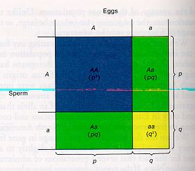
Fig. 1.4. Distribution of genotypes for a diploid, two-allele system. Note especially the two ways to get heterozygotes (A from mother, a from father vs. a from mother, A from father. That is why we get 2pq in the formula above). Note also that we distinguish between allele names (using labels such as A or a) and their frequencies (p or q). Hardy-Weinberg equilibrium (HWE) is a fundamental premise of population genetics. Deviations from HWE can provide important insights into forces that determine the distribution of variation in natural populations.

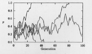
Fig. 1.5. Computer simulation of genetic drift. The frequency of an allele (e.g., A in a system with A and a) is shown for five replicate populations over the course of 100 generations, with a population size (N) of 20. The effect of drift is inversely proportional to population size; drift can be a fundamental driving force in evolutionary divergences. Note that drift is a process with what we call "absorbing boundaries". Once p reaches either 0 or 1 it cannot change (barring an extrinsic process such as mutation or genetic migration). Thus all alleles in finite populations head inexoprably toward fixation or loss. The smaller the N, the faster the march toward the boundaries.

Fig. 1.6. Microsatellite allele frequencies for three populations of black bears in Wyoming. Note that SE WY (Snowy Range) has low frequency of the purple allele (207 bp; here we are are labeling the alleles according to their size in base pairs, bp) but high frequency of the light blue allele (205 bp). The converse is true for the two populations in NW WY.

We can also use population genetics principles to assign individuals (probabilistically) to a source population even after they have dispersed and been sampled in another location.

Fig. 1.7. Assignment test graph for black bears from NW WY (Black Rock, blue diamonds) and SE WY (Snowy Range, pink squares). Individuals falling above the diagonal have a higher likelihood of "being from" the Snowy Range, those below the diagonal have a higher probability of being from Black Rock. Note that one bear sampled at Black Rock (UA195, a male) is "assigned" to the Snowy Range, suggesting that he may be a disperser or the descendant of a recent immigrant. Two bears sampled in the Snowy Range (Ua 081, a female, and Ua 105, a male) cluster with the Black Rock population. We therefore have evidence of population structure (most bears "belong" to the locality where they were sampled) but also have evidence of INDIVIDUALS who may have dispersed or at least have genotypes more typical of another population.

We can use population genetics results for comparative studies. In the example below I compared some allozyme results for Florida scrub endemic plants to means for a wide series of ecological and taxonomic categories in a meta-analysis by Jim Hamrick of the U. of Georgia.

Fig. 1.8. Degree of allozyme polymorphism (P_S) for three kinds of scrub plants in Florida - four species of rare mints in the genus Dicerandra; Eryngium, a rare endemic in the family Apiaceae; and Ceratiola, an endemic in the Empetraceae (its only North American confamilial is the boreal crowberry Empetrum). Take-home points include the fact that polymorphism of Eryngium is low compared to means for categories such as endemics, selfing plants, and short-lived dicots. In contrast, the Dicerandra species, despite being very rare and having very narrow ranges (one species is now known only from a few hectares along the Atlantic coast of Florida) show reasonably high levels of polymorphism.

Individualization, relatedness: We will then turn to fine-grained analyses of genetic variation. In some cases, fundamental principles of population genetics play a role (for example, analyzing levels of relatedness among individuals has clear roots in classical population genetics analysis of inbreeding), while in other cases newer techniques exist, based on the very high levels of variation found with some genetic markers (such as DNA fingerprints — mini satellites-- or microsatellites).

Conservation and management applications: Finally, we will see how all three of the major levels we addressed in the course —

phylogenetics and systematics

population genetics

fine-grained individual identity and relatedness

can be brought to bear on problems of conservation and management.

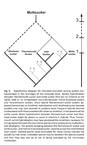
Example: With Tom Parchman (who will do some guest lectures), former UW graduate student and BLM biologist Mike Bower, and Drs. Wayne Hubert and Frank Rahel of the department of Zoology, I looked at genetic variation in native fishes of the Muddy Creek drainage south of Rawlins (part of the Colorado River system). One of the disturbing things we found is that an introduced species, the white sucker (Catostomus commersoni) has hybridized readily with native flannelmouthg suckers (C. latipinnis). The hybrids, in turn, have been able to hybridize with oanother native species the bluehead sucker (C. discobolus). Even worse, other native species are closely enough related to the white and flannelmouth suckers that they will likely be drawn into the "muttsucker" mixture. Below is the figure from our recent paper, showing the proposed phylogenetic consequences of this hybridization (McDonald, D.B., T.L. Parchman, M.R. Bower, W.A. Hubert, and F.J. Rahel. 2008. An introduced and a native vertebrate hybridize to form a genetic bridge to a second native species. Proceedings National Academy of Sciences, USA 105: 10842-10847).

The molecular tools: I will now start using some technical jargon with which we will become familiar later. Don’t worry too much about definitions at this point, the main point is to get a sense of the wide array of molecular tools at our disposal. The molecular tools that we will bring to these portions of the course include protein products analyzed on electrophoretic gels (allozymes), microsatellites (simple sequence tandem repeats such as AC repeated 20 to 30 times), and AFLP (amplified fragment length polymorphisms).

Fig. 1.10. Stylized diagram of an electrophoretic gel for microsatellites. A current draws amplified DNA down "lanes" in the polyacrylamide gel. The fragments can then be separated by size (bp = base pairs) and individuals can be genotyped for their allelic composition (homozygote or heterozygote for one or more alleles). Here the left-hand lane has a "ladder" of known-size fragments, the second lane has the DNA from one individual (genotype bc =131/133) and the third lane has the DNA from a second individual (genotype ad = 129/137). Running multiple loci provides a wealth of genetic information about individuals, populations or species.

Fig. 1.11. Representative microsatellite and gender probe gel. DNA was amplified by PCR and run out on a Li-Cor automated sequencer for scoring by fragment size (number of base pairs).

Other molecular marker tools include minisatellites (longer, more complex tandem repeats with large interindividual length variation), sequences of base pairs in the nuclear genome or in mitochondrial DNA (mt-DNA), and RFLP’s (restriction fragment length polymorphisms) -- variation exposed by restriction enzymes that cut DNA at specific sequences.

These days, most of the DNA analyses done by evolutionary biologists working on natural populations will do their genetic analyses on an automated "sequencer". Here at UW, that means an ABI machine that runs the DNA through capillary tubes and "visualizes" the fragments with laser beams. The depictions above of "gel lanes" are therefore an analogy, not a literal depiction of the process -- but the analogy works, because the fragments still move through the capillary at different rates and are detected in passing by the laser.

** This section will be web-only ** Please review before class on Weds., if possible

Before we delve into phylogenetic techniques and the molecular tools we use to obtain phylogenetically informative data, let’s do a quick review of some basic genetics. I strongly recommend that, if it’s been a while since you took genetics, you review a basic text on molecular structure, mitosis and meiosis, Mendelian inheritance and the like.

The basic structure of DNA: Here I provide a summary of what I see as absolutely essential basic knowledge. Most of the students who take this course are probably most interested in diploid (two sets of chromosomes, one paternal the other maternal) or polyploid (multiple sets of chromosomes, found mostly in plants -- plus one South American rodent!) organisms. Nevertheless, some of the tools for analyzing populations are haploid (mt-DNA, pollen grains, sperm, unfertilized eggs, haploid male Hymenoptera). DNA has four kinds of building blocks, the nucleotides: A, G, C, and T. The nucleotides differ in their nitrogenous bases. A and G are purines, while C and T (and U for RNA) are pyrimidines. [Purine or pyrimidine nitrogenous base + ribose or deoxyribose sugar + phosphate group = nucleotide]. When one gets to sequence data and the generation of point mutations the terms transition and transversion often come up. Transitions involve purine to purine or pyrimidine to pyrimidine (i.e., like to like) and seem to occur more frequently than transversions (change to unlike). Some phylogenetic methods involve character weightings for the relative likelihoods of transitions vs. transversions. A chromosome consists of two complementary strands of DNA — the sense and antisense strands. The strands are arranged in an intertwined double helix configuration. Each base pair (the A,G, C or T are base pairs) has an orientation along the strand — a 5’ ("five prime ") group at one end and a 3’ ("three prime") group at the other. When we get to the polymerase chain reaction (PCR), for example, we will be talking about 3’ and 5’ orientation. When the genetic code is translated into proteins, the mRNA reading goes from 5 ’ to 3 ’. During meiosis and mitosis, replication turns single strands of DNA into double strands by the process of complementarity. Each base pair matches up with its complement -- A with T, C with G -- to regenerate a double strand from a single strand.

Coding and non-coding stretches: A chromosome’s genes consists of portions that will be turned into protein product (exons) but also includes parts that are transcribed but not translated into proteins (introns), as well as long stretches not associated with any kind of gene (e.g., the satellite "junk" DNA usually found near the centromeres of chromosomes). At first glance one might think that the only interesting parts are the expressed genes. In fact, though, much of what we will address in this course deals with non-coding DNA. The microsatellites that are my major molecular tool are non-coding stretches of very simple motifs (AC repeated 20 to 30 times in different individuals’ chromosomes, or AGT repeated 12 to 25 times ).

Mendelian inheritance: Diploid organisms have two copies of each type of chromosome (the chromosome complement or karyotype number varies across diploid organisms from as few as 4 in Drosophila fruit flies to as many as 80 in a Nymphaea fly --humans have 23 different kinds. Chromosomes also vary great in size. Birds, for example, have many tiny microchromosomes -- these tend to prevent the physical linkage disequilibrium that can arise in the large chromosomes of mammals. Each parent (mother and father) contributes one of its pairs of chromosomes to make up the complement in its offspring. Because of the process of independent assortment, offspring will receive differing combinations of the paired chromosomes (except for identical twins and clones). Given 23 chromosomes and independent assortment, each human can produce 2²³ combinations of chromosomes in her or his gametes -- more than 8 million possible types. Different chromosomes can have different stretches of DNA sequence at the same place (locus) on a particular chromosome. These variants are known as alleles. You may tend to think of alleles as referring exclusively to expressed (coding) portions — they can however, refer to any stretch of DNA at which we can find variation. Indeed non-coding microsatellite alleles will be the stuff of much of what we do in the population genetics section. The occurrence of two different alleles on the two homologous chromosomes produces the familiar possibilities of genotypes AA (both mom and dad contributed a "big A"), Aa (mom or dad contributed a "big A", the other parent a "little a") or aa (both mom and dad contributed a "little a"). (Fully) recessive alleles are expressed only when present as homozygotes (aa = white, AA and Aa = red). Genes or markers can be either dominant or codominant. With codominant markers, the heterozygotes show an intermediate or distinguishable-from-either-homozygote phenotype (aa = white, Aa = pink, AA = red; 129/129 shows one band, 129/131 shows two bands, 131/131 shows one band on an electrophoretic gel). Codominance will be very important even for our non-coding microsatellites because the variants differ in size. A homozygote will show just one band (we can sometimes tell it is doubled by the density of the visualizing agent), whereas heterozygotes will show two different bands. With a dominant marker, the heterozygotes do not show a distinct phenotype, and one must therefore make assumptions in order to estimate critical parameters such as the heterozygosity. As a result, dominant markers such as RAPDs and AFLPs present analytical challenges when we wish to conduct classical population genetics analyses with the output data. Nevertheless, the power of having hundreds of AFLP loci vs. a few microsatellite loci, provides power that more than compensates for the disadvantages in many analyses.

As a contrast to the pattern of Mendelian inheritance, mitochondria are maternally inherited clones. The distinction has important ramifications for making inferences. For example, the effective population size is smaller, and the lineages are inherently better-suited to the dichotomous branching pattern of lineages used in cladistic analyses.

Mutations: The most familiar type of mutation is a point mutation -- during replication a different nucleotide is placed in the chain (say an A, G, or T instead of the original C). Point mutations occur at a low rate (approximately 10-6 or once in a million replication events). A key point is the transition/transversion distinction mentioned above. Microsatellites (my almost exclusive tool) generally do not mutate by point mutations. Instead a process of slippage replication adds or subtracts the beads on the necklace so that we go from AC₂₀ to AC₁₉ or AC₂₁ or from GCC₁₈ to GCC₁₇ or GCC₁₉. It appears that the most common "mutation" is the addition or subtraction of a single repeat unit. This means that mutation is a "stepwise" process and, in theory, provides phylogenetic information. That is, all things being equal (in practice, they rarely are) alleles that are more similar in size are more closely related to one another than alleles with a wider size disparity.

Return to top of page