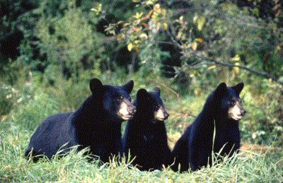
Fig. 9.1. Black bears. Presence or absence of the 205 or 207 alleles at Locus G1A is virtually diagnostic of whether the bears come from NW or SE Wyoming.
Return to Main Index page
Go to discussion/example of Assignment test
Black bears in Wyoming are restricted to montane forest habitats. The intervening prairie, grassland or shrub-steppe habitats that make up much of the landscape are unsuitable habitat, and may act as major barriers to gene flow, allowing populations to diverge in gene frequencies. My graduate student, Michael Cachelin and I used microsatellites to look at the population structure of three Wyoming black bear populations (Fig. 1). The Black Rock (Tetons) area in the northwest, the Big Horns in north-central Wyoming, and the Snowy Range in southeast Wyoming.
Fig. 9.1. Black bears. Presence or absence of the 205 or 207 alleles at Locus G1A is virtually diagnostic of whether the bears come from NW or SE Wyoming.
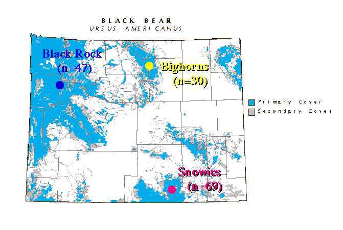
Fig. 9.2. Location of study populations in Wyoming. Throughout,
blue fonts or symbols will refer to the Black Rock/Tetons population (NW),
yellow fonts to the Big Horns population (N central)and pink/reddish to the Snowies population (SE).
We genotyped 30 or more bears from each population at four polymorphic loci developed by Canadian researchers. The four loci and the number of alleles per locus were as follows:
Locus Alleles per locus
If we look more closely locus by locus we see thatG1A 6 alleles (range/pop. 3-5)
G10C 6 alleles (range/pop. 3-5)
G1D 8 alleles (range/pop. 4-7)
G10L 16 alleles (range/pop. 8-12)
1) gene frequencies and the evenness of allele frequencies vary greatly between populations
2) the allele frequencies have large gaps between size ranges
(under a strict SMM stepwise mutation model we would expect a bell-shaped distribution)3) the loci vary greatly in number of alleles (presumably reflecting differences in the mutation rate across loci)
Here are the values for gene diversity (or expected
heterozygosity: He or D) and the
effective number of alleles, Ae (calculated as [1/(1-Di)]/4
-- i = 1 to 4).
N.B. We do not get Ae right if we calculate it from the overall He shown in the table below. We have to do it locus by locus.
An interesting way to look at the data is to use an assignment test. Essentially, this involves taking the logarithm of the joint probability of a given genotype in the population from which it was sampled, versus the probability in another population. Let�s do a simple example with three genotypes from two populations at three slightly polymorphic loci.He Ae
_____________________________Snowies 0.53 2.67
Black Rock 0.61 3.09
Big Horns 0.64 3.24
______________________________
Gene frequencies for two populations at three loci.
| Gene frequency | |||
|
|
|
|
|
|
|
|
|
|
|
|
|
|
|
|
|
|
|
|
|
|
|
|
|
|
|
|
|
|
|
|
|
|
|
|
|
|
|
|
|
|
|
|
|
|
|
|
|
|
|
|
|
|
|
|
|
|
|
|
Now we look at the genotypes of three individuals
and the site where they were sampled:
|
|
Genotype | Sample site |
|
|
ab/bc/cc |
|
|
|
aa/ac/cd |
|
|
|
cc/ab/cc |
|
Now we can calculate the log likelihood that each
of the three individuals "belongs" to population 1.
We do so by multiplying the population
frequencies (in Pop 1) for the genotypes of the individuals. (Here I ignore the complication that we should adjust the population frequencies of an individual in its sampled population by removing it from the pool before calculating the gene frequencies).
|
|
Formula |
|
||||
|
|
Pop1= | Ln(2*0.25*0.1*2*0.15*0.05*0.75*0.75) |
|
|||
|
|
Pop1= | Ln(0.25*0.25*2*0.8*0.05*2*0.75*0.1) |
|
|||
|
|
Pop1= | Ln(0.5*0.5*2*0.8*0.15*0.75*0.75) |
|
|||
Then do the same thing for "belonging" to Pop. 2.
|
|
Formula |
|
||||
|
|
Pop 2 = | Ln(2*0.4*0.3*2*0.2*0.3*0.25*0.25) |
|
|||
|
|
Pop 2 = | Ln(0.4*0.4*2*0.5*0.3*2*0.25*0.35) |
|
|||
|
|
Pop 2 = | Ln(0.1*0.1*2*0.5*0.2*0.25*0.25) |
|
|||
Let�s see exactly how we got -9.1571 for Individual 98-001 in Pop. 1. Its genotype was ab at Locus 1. The gene frequency of a in Pop. 1 was 0.25, of b was 0.1. Multiply the two together (the joint probability of having an a AND a b allele), then multiply by two (because we can get heterozygotes two ways). Now do the same for the other two loci (note that the homozygote probability for the third locus is NOT multiplied by two). Take the natural logarithm of all that. What we will compare that number to is the value for the same individual using the other population�s gene frequencies. That gives us the log-likelihood of assigning Individual 98-001 to each of the two populations. We "assign" it to the population in which it has the highest (least negative) log-likelihood.
Why are three of the log likelihood boxes colored yellow? Those are the highest (least negative) values for that individual. Individual 98-001 is most likely to have come from ("is assigned to") Population 2. So is Individual 98-002. Individual 98-003 is most likely to have come from Pop. 1. Wait a second, though! Individual 98-002 was collected/sampled from Pop. 1. The assignment test "mismatch" may point to the possibility that this individual was a disperser from Pop. 2 (where it was born and got the Pop. 2 "genetic signature") to Pop. 1 (where it was sampled).
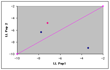
Fig. 9.3. Plot of log-likelihoods for a simple three-individual assignment test. The line of equality separates the assignment areas. Individuals that fall above the line are "assigned" to Pop. 2, those below the line to Pop. 1. The individual in pink was sampled in Pop. 1 but has a higher assignment probability to Pop. 2.
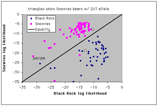
Fig. 9.4. Assignment of individuals to populations by log-likelihood profiles. Three bears sampled in the Snowies and two bears sampled in the Black Rock/Teton area have profiles that affiliate them with the other population - these might represent immigrants to the populations or the descendants of recent immigrants. Triangles mark the two Snowy Range bears with the 207 bp G1A allele (the only occurrences in the Snowies population).
PCAGen available for Windows platforms from:
and several other interesting variants, including a Bayesian assignment test from:
http://www.montpellier.inra.fr/URLB/geneclass/geneclass.html GENECLASS for Windows. GeneClass is a program for assignation and exclusion using molecular markers (similar to, but more diverse than Paetkau assignment testing)
Let�s look now at several different measures of population differentiation. These will be either variance-based measures (such as F-statistics) or distance measures (such as Cavalli-Sforza chord distances). Some will be based on a stepwise mutation model (SMM), others on an infinite alleles model (IAM), while yet others such at the Cavalli-Sforza distance are not based on any underlying biologically based model.
First, let�s look at a set of pairwise comparisons with FST values:
FST (IAM)
Snowies-Big Horns 0.27
Snowies-Black Rock 0.31
Black Rock-Big Horns 0.03
These data tell us that the Snowies are well differentiated from both of the northern populations, but that the differentiation between the Black Rock/Teton area is much less pronounced. Both on the basis of simple geographic distance and on the basis of other biogeographical evidence I will come to later, this makes pretty good sense.
Now let�s examine a variance-based SMM measure, the RST of Slatkin (1995) as modified by Goodman (1997).
RST (SMM)
Snowies-Big Horns 0.40
Snowies-Black Rock 0.15
Black Rock-Big Horns 0.08
These data give a somewhat similar picture, but show
considerably less contrast between the Big Horns and the Snowies. Next,
let�s look at a distance measure based on allele sizes under the SMM --
Goldstein�s ![]()
(SMM - stepwise)
Snowies-Big Horns 10.05
Snowies-Black Rock 2.29
Black Rock-Big Horns 3.00
These results are difficult to reconcile with the biogeography. It seems very unlikely that the Snowies can be hugely different from the Big Horns, while the Black Rock/Teton area is more similar to the Snowies than the Tetons are to the Big Horns. The problem here is that the strong emphasis on allele size differences (which would greatly downplay, for example, the stark contrast between the Tetons and the Snowies at 205/207 for Locus G1A) leaves little room for detecting the influence of drift. Even if allele distributions under mutation alone were stepwise (and therefore bell-shaped), drift would cause allele distributions to develop gaps and irregularities. Looking back at the allele distribution gaps it is hard to imagine that drift hasn't played an important role in making the allele distributions irregular.
Our final measure will be one based neither on SMM or IAM -- the Cavalli-Sforza chord distance, which is a purely geometric measure that simply takes the numbers at face value and plots them on the surface of a hypersphere (on the surface of a sphere with more than three dimensions).
Cavalli-Sforza chord distance (no biological assumptions)
Snowies-Big Horns 0.15
Snowies-Black Rock 0.13
Black Rock-Big Horns 0.05
Like the FST values, this seems to have the desirable
property of making the distance from the Snowies to either of the other
populations almost equivalent, and considerably larger than the distance
between the Tetons and the Big Horns. Further, it takes account of all
the data simultaneously, whereas FST either incorporates
all the data into a single overall measure of differentiation for all three
populations, or computes pairwise distances by ignoring the data from the
third population. Finally, Takezaki and Nei (1996) used simulated data
to generate phylogenetic trees -- for the sorts of population sizes and
number of loci likely to be the maximum available to students of natural
populations of vertebrates, the Cavalli-Sforza distance performed well.
In contrast, ![]() performed very poorly.
performed very poorly.
Since at least two lines of evidence support the use of the Cavalli-Sforza distances, we will use them to generate a tree that includes gene frequency data for populations of bears in the region (MT, ID and CO) as well as Maine (as an outgroup).
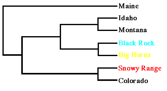
Fig. 9.5. UPGMA tree from Cavalli-Sforza chord distances for three Wyoming black bear populations and samples from surrounding states, with Maine as an outgroup. Note that the Snowy Range population clusters with Colorado, while the northern Wyoming populations cluster with Montana and Idaho.
A final analysis, not directly related to the biogeographic patterns is to make an estimate of relative effective population size (Ne). Unfortunately, population size enters into population genetic equations as part of two kinds of compound terms 4Nem or 4Nem, where m is the mutation rate and m is the migration rate. Unless we know either the mutation or the migration rate we cannot estimate an absolute number for Ne. Nevertheless, we can estimate relative population sizes using the measure Q = 4Nem estimated by Nielsen�s program Misat. Based on that we compute the following relative sizes:
Black Rock : Snowies 1.0 : 0.69 (CI 0.42-1.14)
Black Rock : Big Horns 1.0 : 0.64 (CI 0.39-1.06)
Both confidence intervals overlap one, so we cannot claim that the size differences are statistically different. Nevertheless, the trends are in a direction that seems compatible with the biology of the bears. The Black Rock/Teton area is undoubtedly part of an extensive contiguous stretch of forested habitat suitable for bears. The Snowies and Big Horns, in contrast are relatively isolated from the "mainland" forest patches.
Conclusions:
1) Populations show large differences over short distances
2) Substantial gene flow between Black Rock and Big Horns
3) Near "fixed difference" at locus G1A (205/207) affects stepwise vs. other model outcomes
4) High assignment probabilities for Tetons vs. Snowies
5) Concordant with biogeographic patterns in other taxa showing a large break across the Wyoming Basin and Green River drainage.
References:
Conroy, C.J., and J.A. Cook. 2000. Phylogeography of a post-glacial colonizer: Microtus longicaudus (Rodentia, Muridae). Mol. Ecol. 9: 165-175.
Findley, J.S., and S. Anderson. 1956. Zoogeography of the montane mammals of Colorado. J. Mammal. 37: 80-82.
Paetkau, D., and C. Strobeck C. 1994. Microsatellite analysis of genetic variation in black bear populations. Mol Ecol. 3: 489-495.
Paetkau, D., and C. Strobeck. 1995. The molecular basis and evolutionary history of a microsatellite null allele in bears. Mol Ecol. 4: 519-520.
Paetkau, D., and C. Strobeck. 1996. Mitochondrial DNA and the phylogeography of Newfoundland black bears. Can. J. Zool. 74: 192-196.
Paetkau, D, S.C. Amstrup, E.W. Born, W. Calvert, A.E. Derocher, G.W. Garner, F. Messier, I. Stirling, M. Taylor, Ø. Wiig, and C. Strobeck. 1999. Genetic structure of the world�s polar bear populations. Mol. Ecol. 8: 1571-1584.
Paetkau, D, W. Calvert, I. Stirling, and C. Strobeck. 1995. Microsatellite analysis of population structure in Canadian polar bears. Mol. Ecol. 4: 347-354.
Paetkau-D; Shields-GF; Strobeck-C. 1998. Gene flow between insular, coastal and interior populations of brown bears in Alaska. Mol-Ecol. 7(10): 1283-1292.
Paetkau, D., L.P. Waits, P.L. Clarkson, L. Craighead, and C. Strobeck. 1997. An empirical evaluation of genetic distance statistics using microsatellite data from bear (Ursidae) populations. Genetics 147:1943-1957.
Takezaki, N., and M. Nei. 1996. Genetic distances and reconstruction of phylogenetic trees from microsatellite DNA. Genetics 144: 389-399.