 Eqn 1
Eqn 1
Assessing
genetic structure using codominant, allelic markers
within and
among
populations
(WAAP analysis), meaning of AE
and tips on software-based analyses.
Download WebSoftware.doc list of web software resources
We have looked at the derivations for a number of population genetic parameters (variance-based and distance measures of population structure) and their strengths and weaknesses in the face of various complexities of natural populations (e.g., small and fluctuating population size, variation in the breeding sex ratio). We will now focus on the practicalities of assessing the genetic structure within and among populations -- what measures are essential for any sort of reasonably comprehensive assessment of genetic structure, what programs are available for computing those measures and how do we organize data for analysis?
Here are some of the essential components (adapted from a checklist developed by Jim Hamrick at U. GA):
I. Total variation over the entire set of populations:
Mean P, A, AE,
H.
The values in Part I are calculated with all the samples considered to
constitute a single group.
These ones are calculated population by population, then averaged over
the set of populations.
Differences among populations in the above. Does
one or more populations have unusually high or low values for any of the
above?
Deviations from Hardy-Weinberg expectations (per
locus and population)
Assessment of linkage disequilibrium
Estimates of Ne, effective population
size (4*Ne*m)
Relatedness or allele-sharing matrices
A note on the calculation and uses of AE (effective number of alleles)
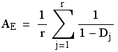
AE is the effective number of alleles (at the level of the OTUs we are examining). Verbally, this measure is the number of equally frequent alleles it would take to achieve a given level of gene diversity. That is, it allows us to compare populations where the number and distributions of alleles differ drastically. The formula is:
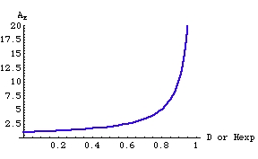
where Dj is the gene diversity of the jth of r loci. Note that we calculate the OTU-level AE by averaging over the AE calculated locus-by-locus rather than by calculating a mean gene diversity and then calculating AE from that. The graph below shows why: AE is a nonlinear function of the gene diversity (Hexp), which brings into play Jensen’s inequality [the expectation of a function ≠ the function of the expectations for nonlinear curves; see Ruel and Ayres (1999)]. Here, because the curve is concave up, the AE we compute will be greater than if we calculated it from the overall gene diversity.
Fig. 1. Effective number of alleles, AE, as a function of the gene diversity (D or Hexp). The nonlinear relationship brings into play Jensen’s inequality. Note that most of the "action" happens for D in the range 0.5 to 0.9 (AE goes from 2 to 10).
The meaning of AE. Say we have two populations (or species, or whatever our OTU is) with the same number of total alleles, but with very different distributions of allele frequencies. We would like to be able to assess the effective number of alleles as a corollary to the expected heterozygosity. Remember that, for any given number of alleles, the expected heterozygosity (gene diversity) is highest when the all the allele frequencies are equal (look at Fig. 5.1 in the web notes). Simply reverse the logic. When the heterozygosity is high (the peak of the curve in Fig. 5.1) we will have the highest effective number of alleles. For a heterozygosity of 0.85 we will have, effectively, 6.7 alleles {formula is AE= 1/(1-Hexp)}. If a locus has 8 total alleles (meaning a maximum possible Hexp of 0.875), but the Hexp is only 0.6, the effective number of alleles will be only 2.5. This tells us that we have a set of alleles with very different frequencies. Alleles with frequencies away from the even “average” contribute very little to the effective number of alleles. When will the effective number of alleles be the same as the actual number of alleles? At the maximum gene diversity (peak of the curve). When will it be at a minimum (near 1)? When one allele (the only real contributor to the effective allele number) dominates the allele frequencies and all the others are very rare. Imagine that one OTU has 10 total alleles, another just 4; they could have the same effective number of alleles, if the allele frequencies are very unbalanced in the first case and much more balanced in the second case. Because of the reciprocal nature of the formula, if the OTUs have the same AE, they will have the same Hexp. That is, if AE1 = AE2, then Hexp1 = Hexp2.
Source: Weir (1990) pp. 124-125
Jensen’s inequality is described in Ruel, J.J., and M.P. Ayres. 1999. Jensen’s inequality predicts effects of environmental variation. TREE 14: 361-366. * For non-linear curves, mean of functions is not same as function of means. Means that variance affects expected outcome/return. Implications for mean-variance tradeoffs, optimal foraging, risk prone vs. risk averse strategies. (Ruel and Ayres overlook a fairly extensive literature on the subject, including classics by Gillespie 1977, MacArthur 1967}.
Some useful software and tips on running it
I begin with a worksheet that has
the data in whatever format I find most useful for genotypes, individual
IDs, population labels, etc. I then create a "starter" two column-format
MS Tools worksheet.
First line has Locus names in 2nd,
4th, 6th etc. columns
Second line has Pop. name and individual's number
in 1st column (you may want to paste this concatenated code
into your "original" sheet so that you can easily check correspondence
between the ID label used for MS Tools and whatever you actually use).
Next column is bp size of first allele, first locus,
then 2nd allele, 2nd locus, etc.
Once you have this set up, go to "Tools" menu bar
and scroll down to "Microsatellites". Note that you first need to select
the kind of data in the top dialog box. (For the example above, we would
have diploid, two-column format).
You can then check for errors, use the Help file,
create other data input formats etc. If you don't get a dialog box for output choices, it means that Toolkit isn't recognizing the data format.
Hints:
a) Remember that pop. names must
be padded to at least 10 spaces.
b) For entering gene freqs (a long string of numbers),
it is definitely best to set it up in a labeled Excel worksheet (using
borders around sets of alleles per locus and labels above, etc.) and then
save the bare-bones data parts as a text-only file. Edit the file a little
more in Word, if necessary.
c) Toggle among choices by typing in the appropriate
characters. (Is your input matrix square or lower-diagonal?).
d) When in doubt, try reading the documentation!
3) FSTAT, GenePop, GDA, TFPGA, Genetix, Arlequin, Identix, Structure, Partition et al. Lots of choices for software that will calculate a wide array of pop. gen. measures. See my "Web genetic software" sheet for a reasonably current list of descriptions and URLs.
4) TreeView.Steps for computing genetic distances using PHYLIP�s GenDist subroutine:
We will start by seeing how to build the input file for computing genetic distance measures from gene frequency data. The software will be the GenDist subroutine of J. Felsenstein�s PHYLIP package. The outputs will be distance matrices between each of the 8, 5 or full 13 populations and each of the others. The three possible distance measure are:
Nei�s genetic distance. [Nei, M. 1972. Genetic distance between populations. Am. Nat. 106: 283-292]
Reynolds� distance. [Reynolds, J., B.S. Weir, and C.C. Cockerham. 1983. Estimation of the coancestry coefficient: Basis for a short-term genetic distance. Genetics 105: 767-779].
i) Copy then rename the formatted file as "infile", which you will put in the same folder (directory) as the GenDist application icon (GenDist.exe file). "Infile" should contain the following information (the text below is taken from the file GenDist.Doc, which is in the documentation folder in the folder for PHYLIP):
The input to this program is standard and is as described in the Gene Frequencies and Continuous Characters Programs documentation files. It consists of the number of populations (or species), the number of loci, and after that a line containing the numbers of alleles at each of the loci. Then the gene frequencies follow in standard format. {If I don't provided the file you could adapt an Excel genotype file to this format}.ii) Double-click the GenDist application icon (ask what folder it is in, if necessary). You will see the following screen:So, for example, we would take out the "Locus" and "Allele" column headers from the Excel file, so that the file contains only the info. Listed in the paragraph above.
Genetic Distance Matrix program, version 3.5p
Settings for this run:A Input file contains all alleles at each locus? One omitted at each locusN Use Nei genetic distance? Yes
C Use Cavalli-Sforza chord measure? No
R Use Reynolds genetic distance? No
L Form of distance matrix? Square
M Analyze multiple data sets? No
O Terminal type (IBM PC, VT52, ANSI)? ANSI {This is irrelevant}
1 Print indications of progress of run? Yes
Are these settings correct? (type Y or the letter for one to change)iii) Once you have the settings correct (e.g., toggle the "A" choice because our data will NOT having a missing allele frequency, hit the "C" toggle to get Cavalli-Sforza chord distance), then type "Y" and carriage return.The A option is described in the Gene Frequencies and Continuous Characters Programs documentation file. As with CONTML, it denotes whether all alleles are represented in the gene frequency input, or whether one one allele frequency has been left out per locus.
C, N, and R denote whether to calculate the Cavalli-Sforza, Nei, or Reynolds et al. genetic distances respectively. The Nei distance is the default, and it will be computed if neither C nor R is explicitly invoked.
The L option denotes whether the distance matrix is to be written out in Lower triangular, Upper or Square form.
The M option is the usual Multiple Data Sets option, useful for doing bootstrap analyses with the distance matrix programs.
iv) You will generate an output file named "outfile", which will be a text-only file that can be opened by a word-processing program.
The output file's first line is simply the number of species (or populations). Each species (or population) starts a new line, with its name printed out first, and then the genetic distances (number of distances per line depends on which of the matrix output options you chose). This output in the standard format used as input by the distance matrix programs. That is, the output, in its default form, is ready to be used in the distance matrix programs.Open the file with Word, add any comments you think appropriate and save it under a different name in a folder of your outputs. Then rename the original as "infile" for use with the next step.
v) ALSO� the outfile (distance matrix) can be
directly used as "infile" for one of PHYLIP�s tree-building routine Neighbor.
[See just below for "Steps for computing NJ and UPGMA trees from genetic
distance matrices"].
vi) You can use the subprogram SeqBoot with the original gene frequency infile to generate 1000 bootstrapped gene frequency data sets. Then do all the normal steps for Cavalli-Sforza distance matrices and neighbor-joining/UPGMA trees, remembering to toggle M for multiple data sets.
i) Generate or obtain a text-only distance matrix file [see "Steps for computing genetic distances using PHYLIP�s GenDist subroutine" above, or use some other method such as obtaining a published distance matrix]. If you did the above, you can begin with a text-only file that is the output from PHYLIP�s GenDist computation. Default (easiest way) is to have the input file distance matrix labeled "infile". Proceed as follows:
ii) Double-click the Neighbor application icon (ask where it is, if necessary).
OPTIONS
Here are some of the options available in all three programs (Kitsch, Fitch and Neighbor). They are selected using the menu of options.
-indicates that negative segment lengths are to be allowed in the tree (default is to require that all branch lengths be nonnegative). This option is not available in NEIGHBOR.
L
indicates that the distance matrix is input in Lower-triangular form (the
lower-left half of the distance matrix only, without the zero diagonal
elements).
R
indicates that the distance matrix is input in uppeR-triangular form (the
upper-right half of the distance matrix only, without the zero diagonal
elements).
{No for both of these means a square matrix}
M is the usual Multiple data sets option, available in all of these programs. It allows us (when the output tree file is analyzed in CONSENSE) to do a bootstrap (or delete-half-jackknife) analysis with the distance matrix{ programs. Toggle this when going the bootstrap route.
The numerical options are the usual ones and should be clear from the menu.
iv) Open your "outfile" with a word processor and save under another name somewhere else. You can then use the topology and branch lengths to construct a more polished-looking tree in some other program (e.g., PAUP, MacClade, plus a drawing/painting program, as described below). Even better, use TreeView to produce a nice tree from your "treefile".
Some introductory references and primers:
Brookfield, J.F.Y. 1996. Population genetics. Curr. Biol. 6: 354-357.
Gillespie, J. H. 1998. Population Genetics: A Concise Guide. The Johns Hopkins University Press, Baltimore, Md.
Hall, B.G. 2001. Phylogenetic Trees Made Easy: A How-to Manual for Molecular Biologists. Sinauer, Sunderland, MA.
Hartl, D.L. 1999. A Primer of Population Genetics (3rd ed.). Sinauer Associates, Sunderland, MA
Amos, W. 1999. Two problems with the measurement of genetic diversity and genetic distance. Pp. 75-100 In Genetics and the Extinction of Species (L.F. Landweber, and A.P. Dobson, eds.). Princeton Univ. Press, Princeton.
Gaggiotti, O.E., O. Lange, K. Rassmann, and C. Gliddon. 1999. A comparison of two indirect methods for estimating average levels of gene flow using microsatellite data. Mol. Ecol. 8: 1513-1519.
Kalinowski, S.T. 2002. Evolutionary and statistical properties of three genetic distances. Mol. Ecol. 11: 1263
Luikart, G., and P.R. England. 1999. Statistical analysis of microsatellite data. TREE 14: 253-256.
Neigel, J.E. 2002. Is FST obsolete? Conservation Genetics 3: 167?173, 2002. (critique of Whitlock and McCauley, 1999).
Paetkau, D., L.P. Waits, P.L. Clarkson, L. Craighead, and C. Strobeck. 1997. An empirical evaluation of genetic distance statistics using microsatellite data from bear (Ursidae) populations. Genetics 147:1943-1957.
Ruzzante, D.E. 1998. A comparison of several measures of genetic distance and population structure with microsatellite data - bias and sampling variance. Can. J. Fish. Aquat. Sci. 55: 1-14.
Takezaki, N., and M. Nei. 1996. Genetic distances and reconstruction of phylogenetic trees from microsatellite DNA. Genetics 144: 389-399.
Tomiuk, J., B. Guldbrandtsen, and V. Loeschcke. 1998. Population differentiation through mutation and drift: a comparison of genetic identity measures. Genetica 102-103: 545-558.
Whitlock, M.C., and D.E. McCauley. 1999. Indirect measures of gene flow and migration: FST not equal to 1/(4Nm + 1). Heredity 82: 117-25. (see critique by Neigel, 2002, of the high Nm = 50 used in their simulation).