![]() (Eqn 5.1)
(Eqn 5.1)
[I will not use indexing for the summations after this -- it will always be summing over i = 1 to n].
See web page with some practicalities of assessing genetic population structure
Download guide to using Exel add-in Microsatellite Toolkit and program FStat on campus computers
Go to web page describing how to calculate FST from heterozygosities (FST.html)
Go to Part B. PHSC view of FST.
Go to Part C. Wahlund meets PHSC.
Part A of this web page shows that an inevitable consequence of genetic variance among subpopulations (= differences in gene frequencies) is a deviation from the Hardy-Weinberg expected heterozygosity for the population as a whole. The more different the gene frequencies among subpopulations, the greater the overall deficiency of heterozygotes. We will develop the simplest possible mathematical model to describe this "consequence of variance" known as the Wahlund effect.
Part B works from a "sinister force F" (PHSC) angle, using Hardy-Weinberg expectations to get at variance from a different angle -- one that measures the strength of the homogenizing force acting to decrease heterozygosity. At the end we will see that the "sinister force" is FST, which we derived with a rather different approach in another web page.
Part C reconciles the Wahlund and PHSC approaches by showing that variance in gene frequencies enable us to compartmentalize (and compare) genetic structure within and among populations. We will see that all of the above examine variance, and that the common statistical approach is F-statistics -- a very general statistical approach to partitioning variance that was developed for statistics applications (not including genetics) and only later applied to population genetics by Sewall Wright (1968).
Our ultimate goal -- to be able to describe patterns of genetic divergence and variation, and to understand the processes that drive those patterns.
A. The Wahlund effect -- reduction of heterozygosity as populations diverge
Imagine a single locus, two-allele system (A, a) with the population organized as n subpopulations each of the same size (N), with gene frequencies p1, p2, p3, p4,�.pn. Notation alert: We are using pi here to distinguish the frequency of just one allele (say, "big A") across n subpopulations. Population genetics is full of overlapping notation -- one must always be aware of the context.
The mean of the subpopulation pi gene frequencies will then be:
(Eqn 5.1)
[I will not use indexing for the summations after this -- it will always be summing over i = 1 to n].
The variance of p is:
(Eqn 5.2)
[Algebra note. The step above is the same as the footwork involved in rearranging the "calculation" versus first principles definitions of elementary variance whereby
(Eqn 5.3)
where the right hand side (RHS) is like the more convenient calculator form (because you can build it from easier pieces)].
Note the interesting fact that Varp = Varq (see Fig 5.1 for a graphical view of the reason, based on a symmetrical concave-down curve). Next, use a Hardy-Weinberg approach to the gene frequencies to get the following expectation for genotype frequencies among subpopulations:
( Eqn 5.4)
The notation E{AA} means the "expected frequency of the AA genotype". We did two steps here. First, a Hardy-Weinberg p2 (with more elaborate notation) for the middle equivalence (the one between the equals signs), then a rearrangement of Eqn 5.2 to get the final term. Convince yourself that the last step is correct by rearranging the beginning and end of Eqn 5.2. Now do the same thing for the expectation for the heterozygotes
(Eqn 5.5)
This is a slightly more complicated substitution/rearrangement job on Eqn 5.2.
Remember that q = 1 - p.
For the second step (middle term) remember that p * q = p * ( 1 - p) = p - p2.
For the last equivalence, note that the " Spi2/n" term at the end of the brackets in the middle, is also part of Eqn 5.2.
By rearranging Eqn 5.2, we get -Spi2/n = -- Varp, which can then be substituted in above to get 2( Spi/n -
but Spi/n =(by Eqn 5.1) so the line above rearranges as
2(- 2Varp(because
and all of that gives us the final term.
The key point in Eqn 5.5 is that the heterozygosity (2
![]() *
*![]() )
now has a negative expression following it
-- a negative variance term. Any variance
in the frequencies of p across subpopulations drags down the heterozygosity
overall. In contrast, each of the homozygosities has a positive
variance term. Any variance in the frequencies of p
across subpopulations will increase the homozygosity overall. The
negative 2*variance taken away from the heterozygotes is balanced by single
variance added to each of the two types of homozygotes. This impact of the variance on the expected genotype frequencies
is called the Wahlund effect.
)
now has a negative expression following it
-- a negative variance term. Any variance
in the frequencies of p across subpopulations drags down the heterozygosity
overall. In contrast, each of the homozygosities has a positive
variance term. Any variance in the frequencies of p
across subpopulations will increase the homozygosity overall. The
negative 2*variance taken away from the heterozygotes is balanced by single
variance added to each of the two types of homozygotes. This impact of the variance on the expected genotype frequencies
is called the Wahlund effect.
Procedure for E{aa} is the same as for E{AA} of Eqn 5.4 except that it will involve q and Varq.
What the Wahlund effect does. If you sample from subpopulations that have diverged sufficiently, you will observe an overall deficiency of heterozygotes. Simplest qualitative intuition may come from thinking of populations fixed for different alleles (expectation of fixation = frequency of allele in source, starting or founder population). The overall expected heterozygosity will reflect the presence of numerous alleles, but each is fixed in its own subpopulation (all individuals are homozygotes) so the globally "expected" heterozygotes never occur. Obviously, when all subpopulations have the same gene frequencies no variance among subpopulations exists, and no Wahlund effect occurs (and FST = 0).
Converse (called "Isolate breaking"): when isolated populations make contact and interbreed we may see a temporary excess of heterozygotes (all first-generation [F1] offspring must be heterozygotes when parents are fixed for different alleles).
Thought experiment to assess understanding. For subpopulations
with a ![]() = X,
what is the expected variance (hint: in terms of X)?
= X,
what is the expected variance (hint: in terms of X)?
Answer [X*(1-X)].
Look back at Eqns 5.2 and 5.3. More details on the answer below, when we reconcile
Wahlund with PHSC-FST.
Source: Elseth and Baumgardner, 1981, pp. 507-508. [I changed their fi notation to make the
derivation of the variance more like the standard statistical formula].
_________________________________________________________________________________________
B. PHSC view of F-statistics
(PHSC is an acronym for Probability of Homozygosity due to Special Circumstances)
Consider three genotypes, AA, Aa, and aa, as before.
Now, imagine a sinister force, F, that is increasing homozygosity.
How can we generate genotypes, given ![]() and
and ![]() ?
We will use a probabilistic approach based on sequential selection of alleles
to make genotypes. This requires remembering that independent probabilities
are multiplicative, while mutually exclusive probabilities are additive.
?
We will use a probabilistic approach based on sequential selection of alleles
to make genotypes. This requires remembering that independent probabilities
are multiplicative, while mutually exclusive probabilities are additive.
John and Susan are in the room.
Probability of picking John then Susan in two picks WITH REPLACEMENT
is 0.5 * 0.5 = 0.25 (the probability of picking John first is 0.5 and is
independent of the probability of picking Susan the second time; it is
one of four equally likely choices JS, JJ, SJ, SS).
Probability of picking John then (Susan or John) in two picks WITH REPLACEMENT = 0.5(0.5 + 0.5) = 0.5 (first we pick John with probability one-half. Then we can pick either Susan or John, each with probability one half: if we pick one, we can't get both, the probabilities are mutually exclusive. JS or JJ is one of two equally probable choices).
Using a probabilistic approach, how do we generate E{AA}, which stands for the "expectation
of AA"?
First allele will be A, with probability ![]() .
.
Probability that the second allele will be the same as the first by special (sinister) forces of PHSC is F.
The probability that the second allele will be A for no special reason is
1-F
times the frequency of A, which is ![]() .
.
This is an additive OR statement -- either the sinister force is working, with probability F, or it's not, with probability 1-F.
Note that when the sinister force, F, is working we don't need to multiply it by the frequency of A
(![]() ). Take the extreme case, where F = 0. Then the F-stuff just disappears
and we have 1*
). Take the extreme case, where F = 0. Then the F-stuff just disappears
and we have 1*![]() ,
which is our "normal" Hardy-Weinberg expectation for the second A (that is, we wind up with p2).
,
which is our "normal" Hardy-Weinberg expectation for the second A (that is, we wind up with p2).
Put the independent (multiplicative; we will pick an allele with probability ![]() , AND another with probability F + [1-F]
, AND another with probability F + [1-F]![]() ) and mutually exclusive (additive OR statement given above) probabilities together to get the expectation for
frequency of AA as follows:
) and mutually exclusive (additive OR statement given above) probabilities together to get the expectation for
frequency of AA as follows:
(Eqn 5.6)
Multiplicative is
additive is F + (1-F)
Now use the same logic for E{Aa}. First allele = A, with probability
![]() .
Second allele is not subject to sinister
homozygosity with one minus the probability that it is, or (1-F),
and, if no sinister force is acting, it occurs as a with probability
.
Second allele is not subject to sinister
homozygosity with one minus the probability that it is, or (1-F),
and, if no sinister force is acting, it occurs as a with probability
![]() .
Because order is unimportant, we can get this two ways, so
.
Because order is unimportant, we can get this two ways, so
(Eqn 5.7)
E{aa} is mirror of E{AA}.
A rearrangement of Eqn 5.7, to solve for F yields:
(Eqn 5.8)
where the numerator is a measure of deviation from Hardy-Weinberg due to our sinister force
(and we will discuss the denominator below).
Multiplying top and bottom of Eqn 5.8 gives us an even more "Hardy-Weinberg look"
(Eqn 5.8a)
Note that now we have one minus [the expectation of Aa under the sinister force (= E{Aa}),
over the Hardy-Weinberg expectation for Aa (= 2pq)].
We could rearrange this to get a form that is very similar to what we developed for
F-statistics in Lecture 4 (cf. Eqns 4.5):
![]() (Eqn 5.8b)
(Eqn 5.8b)
That is, we have the difference between two measures of heterozygosity, divided by the first of the two measures.
Source for PHSC: Gillespie, 1998, p. 86
______________________________________________________________________________
Now, let�s reconcile our Eqn 5.7 PHSC approach to E{Aa}
with our Eqn 5.5 Wahlund approach to E{Aa}.
That is, we will set (right-hand-side = RHS of Eqn 5.7) =
(RHS of Eqn 5.5).
(Eqn 5.9)
Rearrange to get F on LHS and everything else on RHS (a 2
Which means that
(Eqn 5.11)
This is cool! Our sinister force (let�s call it FST since we are calculating the variance of subpopulations relative to the total variance) is:
the ratio of the excess homozygosity due to the Wahlund effect (which equals twice the variance in the pi, given by Varp), relative
to the expected overall expected heterozygosity for the whole set of populations, given by 2(which can also be viewed as twice the variance of a binomial variable, which is x(1 - x) or pq), as noted below. [This expected value is the answer to the thought experiment suggested above].
Thus, F-statistics are a way of partitioning variances in gene frequencies among subpopulations by using ratios of different variances. Here we see that one way to think of FST is as the ratio of the Wahlund effect excess homozygosity (2 times the variance of p) to the expected global heterozygosity (twice the variance of a binomial variable). This variance-partitioning basis for F-statistics comes from statistics, and was applied to population genetics by Sewall Wright (1968).
For any given set of ![]() ,
,
![]() {0
<=
{0
<= ![]() <=
1, 0 <=
<=
1, 0 <= ![]() <=
1, and
<=
1, and ![]() +
+![]() =1} the expected variance of pi
=
=1} the expected variance of pi
= ![]()
![]() .
.
Fig. 5.1, below, provides further graphical exploration.
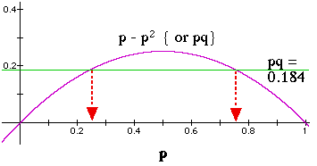
Figure 5.1. Relationship of gene frequencies to variance ( and thereby to expected heterozygosity) for a two-allele system. The graph above was developed for a problem of calculating the allele frequencies when knowing only the heterozygosity, but could apply equally well to calculating the expected variance (Y-axis),
The among-subpopulation variance, Varp, will attain its global (total populations) expected value
Given the heterozygosity, He, and if we have just two alleles, we can solve for the allele frequencies (pq = 0.5*He). In such a case we are moving from a known Y-axis (heterozygosity) to the allele frequencies on the X-axis. [Here I'm solving for 2pq = 2 * 0.184 = 0.386]. Because of the symmetry of the curve and the p+q = 1 property, the alleles will fall equidistant from the centerline (centerline is at p = q = 0.5).
Another way to think of the variance term in the denominator
of Eqn 5.11 is as twice the binomial variance.
Variance of the binomial is n*p(1-p), where n is the "number of trials".
With only one trial (we have only one ![]() and one
and one ![]() for our total population),
the variance = 1*
for our total population),
the variance = 1*
![]() *
*![]() .
.
The three (fundamental) kinds of F-statistics in population genetics:
FIS (inbreeding coefficient, where I stands for Individual and S for Subpopulation).Commonly used variants of FST
(Eqn 5.12)
This F (presented here in Eqn 5.8a form; compare and contrast with form of Eqn 4.5) describes the variance within Individuals, relative to their Subpopulations. It can range from -1 to +1. Consider a simple 2-allele (A, a) system, with p = q = 0.5 in each of two different subpopulations. FIS depends on the ratio of observed heterozygotes (HI is the observed proportion of heterozygotes in the subpopulation) to the expected (HS = average 2piqi via Hardy-Weinberg -- note the averaging bar over the 2piqi in the denominator). If subpopulation 1 has no heterozygotes, then we have 1 minus zero over 0.5 = 1 –– meaning the subpopulation is completely inbred. Now take the opposite extreme for subpopulation 2. All the individuals are heterozygotes. That makes HI = 1, 2pq = 0.5, 1 / 0.5 = 2, and so FIS = -1. The population is completely outbred (perhaps we have the first generation after an isolate breaking case, where homozygotes for a subpopulation fixed for A have all mated with homozygotes for a different subpopulation fixed for a, so their offspring are all Aa heterozygotes).
FST (variance among subpopulations, where S stands for Subpopulations and T stands for Total population).
(Eqn 5.13)
This F describes the variance within Subpopulations, relative to the expected variance in the Total population (HT = 2*
FIT is much less commonly used, but follows from the same logic.
Correlation among uniting gametes:
(theta) of Weir and Cockerham (1984)
GST of Nei (1973) (
RST of Slatkin (1995), as modified by Goodman (1997) -- based on a stepwise mutation model
See my "practicalities of analysis" page, which also has a download for "Web genetic software.doc"
Gillespie's (2004) Appendix B provides yet another way to view F-statistics -- as the correlation among uniting gametes. This is close to Wright's (1951) original conception of F as the probability that alleles identical-by-descent (IBD) will be combined in zygotes.
References (Trends Ecol. Evol [= TREE] papers are mostly a launching point):
Further thoughts on gene frequencies, variance and FSTBohonak, A.J. 1999. Dispersal, gene flow, and population structure. Q. Rev. Biol. 74: 21-45.
Bossart, J.L., and D.P Prowell. 1998. Genetic estimates of population structure and gene flow: Limitations, lessons and new directions. Trends Ecol. Evol. 13: 202-206.
Elseth, G.D., and K.D. Baumgardner. 1981. Population Biology. Van Nostrand, NY.
Gillespie, J. H. 2004. Population Genetics: A Concise Guide (2nd edn.). The Johns Hopkins University Press, Baltimore, Md.
Goodman, S.J. 1997. RST Calc: a collection of computer-programs for calculating estimates of genetic differentiation from microsatellite data and determining their significance. Mol. Ecol. 6: 881-885.
Hedrick, P.W. 1999. Perspective: Highly variable loci and their interpretation in evolution and conservation. Evol. 53: 313-318.
Jarne, P. and P.J.L. Lagoda. 1996. Microsatellites, from molecules to populations and back. Trends Ecol. Evol. 11: 424-429.
Luikart, G., and P.R. England. 1999. Statistical analysis of microsatellite data. Trends Ecol. Evol. 14: 253-256.
Nei, M. 1973. Analysis of gene diversity in subdivided populations. Proc. Natl. Acad. Sci. USA 70: 3321-3323.
Neigel, J.E. 2002. Is FST obsolete? Conservation Genetics 3: 167?173, 2002.
Rousset, F., and M. Raymond. 1997. Statistical analyses of population genetic data: new tools, old concepts. Trends Ecol. Evol. 12: 313-317.
Slatkin, M. 1995. A measure of population subdivision based on microsatellite allele frequencies. Genetics 139: 457-462
Weir, B.S., and C.C. Cockerham. 1984. Estimating F-statistics for the analysis of population structure. Evol. 38: 1358-1370.
Whitlock, M.C., and D.E. McCauley. 1999. Indirect measures of gene flow and migration: FST ≠ 1/(4Nm + 1). Heredity 82: 117-25.
Wright, S. 1951. The genetical structure of populations. Ann. Eugen. 15: 323-354.
Wright, S. 1978. Evolution and the Genetics of Populations, Vol. 4: Variability Within and Among Natural Populations.
University of Chicago Press, Chicago. UW library call # QH 341.W79 v.4
1) The largest numerical value of Varp =______________________________________________________________________________2) Furthermore, alleles of equal frequency will be less likely to wander to one of the "absorbing boundaries" 0 or 1 (loss or fixation, respectively). Thus, loci with even mean-over-the-whole-population allele frequencies will tend to be the most "pattern-revealing" because they have greatest numerical scope for variance. Drift, however, might make some alleles fix one way in one population and one way in another, which will also produce pattern.
Material below is Not Required and refers particularly to microsatellite analyses we will come to later in the course.
3) Sampling variance is something we wish to avoid, but "pattern variance" (e.g., FST) is something we seek optimal ways to detect.4) What is the effect of having allele frequencies that are not normally distributed? See Ruzzante (1998) for a discussion of differences among various distance measures even AFTER we determine that the frequencies are normally distributed. Ruzzante worked with huge populations of cod and had sample sizes of > 1000, so some of what he found may not apply to the sorts of small, patchy populations that we are often interested in analyzing with microsatellites (because "chunkiness" problems take precedence in small populations of bears, mountain lions etc.).
5) Given a complete sample of a small population do we have a "sampling problem"? This should relate to the problem of demographic stochasticity -- whereby a small population with few individuals has unitary reproduction (1, 2, 3 or n babies, not 3.754) and survival (0/1 Y/N not annual survival of 89.365%). With small populations we run into the force of drift problem given by 1/2N.
Do some measures perform better than others when dealing with "chunky" allele distributions [non-normal allele distributions in which alleles may be missing or over-represented]?6) Founder effects, bottlenecks and other causes of chunkiness will invalidate the stepwise assumption that size similarity of alleles reflects phylogenetic relatedness. Which non-stepwise measures are most robust to this sort of effect? Various measures now exist for assessing bottlenecks (see Luikart and England, 1999 and programs such as BOTTLENECK from http://www.ensam.inra.fr/urlb).
7) Geometric analyses such as principal components analysis do not allow statistical tests of significance of difference. Can we analogize from CI/stat. tests for geometric pop. gen. distance measures such as Cavalli-Sforza chord distance and Rogers� distance to make tests for PCA, multidimensional scaling etc?
Could we use percentage overlap? Could one bootstrap the data to get CI for % overlap (seems computation intensive)?
References:
Linked question: Can we put populations onto a likelihood ratio plot/assignment graph, as we do individuals?Luikart, G., and P.R. England. 1999. Statistical
analysis of microsatellite data. TREE 14: 253-256.Paetkau, D., L.P. Waits, P.L. Clarkson, L. Craighead, and C. Strobeck. 1997. An empirical evaluation of genetic distance statistics using microsatellite data from bear (Ursidae) populations. Genetics 147:1943-1957.
Ruzzante, D.E. 1998. A comparison of several measures of genetic distance and population structure with microsatellite data - bias and sampling variance. Can. J. Fish. Aquat. Sci. 55: 1-14.
Takezaki, N., and M. Nei. 1996. Genetic distances and reconstruction of phylogenetic trees from microsatellite DNA. Genetics 144: 389-399.