Return to Main Index page

A. What are microsatellites?

B. What uses do microsatellites serve?

C. How we develop microsatellite primers?

D. How do we screen DNA with species-specific or heterospecific primers?

E. What data-analysis tools are available?

Go to primer on microsatellites on Dave McDonald's web page

Microsatellites are simple sequence tandem repeats (SSTRs). The repeat units are generally di-, tri- tetra- or pentanucleotides. For example, a common repeat motif in birds is AC_n, where the two nucleotides A and C are repeated in bead-like fashion a variable number of times (n could range from 8 to 50). They tend to occur in non-coding regions of the DNA (this should be fairly obvious for long dinucleotide repeats) although a few human genetic disorders are caused by (trinucleotide) microsatellite regions in coding regions. On each side of the repeat unit are flanking regions that consist of "unordered" DNA. The flanking regions are critical because they allow us to develop locus-specific primers to amplify the microsatellites with PCR (polymerase chain reaction). That is, given a stretch of unordered DNA 30-50 base pairs (bp) long, the probability of finding that particular stretch more than once in the genome becomes vanishingly small (if the four nucleotides occur with equal probability then the probability of a given 50 bp stretch is 0.25⁵⁰. In contrast, a given repeat unit (say AC₁₉) may occur in thousands of places in the genome. We use this combination of widely occurring repeat units and locus-specific flanking regions as part of our strategy for finding and developing microsatellite primers.  The primers for PCR will be sequences from these unique flanking regions.  By having a forward and a reverse primer on each side of the microsatellite, we will be able to amplify a fairly short (100 to 500 bp, where bp means base pairs) locus-specific microsatellite region.

Mutation process: Microsatellites are useful genetic markers because they tend to be highly polymorphic. It is not uncommon to have human microsatellites with 20 or more alleles and heterozygosities (H_exp = gene diversity, D) of > 0.85. Why are they so variable? The reason seems to be that their mutations occur in a fashion very different from that of "classical" point mutations (where a substitution of one nucleotide to another occurs, such as a G substituting for a C). The mutation process in microsatellites occurs through what is known as slippage replication.  If we envision the repeat units (e.g., an AC dinucleotide repeat) as beads on a chain, we can imagine that during replication two strands could slip relative positions a bit, but still manage to get the zipper going down the beads.  One strand or the other could then be lengthened or shortened by addition or excision of nucleotides.  The result will be a novel "mutation" that comprises a repeat unit that is one bead longer or shorter than the original.  The idea that adding or subtracting one repeat is likely easier than adding or subtracting two or more beads is the basis for using the Stepwise Mutation Model (SMM) as opposed to the Infinite Alleles Model (IAM).  An advantage of the SMM (at least in theory) is that the difference in size then conveys additional information about the phylogeny of alleles.  Under the IAM the only two states are "same" and "different".  Under the SMM we have a potential continuum of different similarities (same size, similar in size, very different in size).  If, however, the SMM does not hold, then we may be worse off using it -- it may actually be highly misleading.   Even if the underlying mutation process is largely stepwise, it is not difficult to see how drift might affect the distribution of allele sizes in a way that would almost entirely invalidate the SMM (visualize this by examining Figs. 6.1 and 6.2 in Lecture 6).  

Advantages of microsatellites as genetic markers:

Locus-specific (in contrast to multi-locus markers such as minisatellites or RAPDs)
Codominant (heterozygotes can be distinguished from homozygotes, in contrast to RAPDs and AFLPs which are "binary, 0/1")
PCR-based (means we need only tiny amounts of tissue; works on highly degraded or "ancient" DNA)
Highly polymorphic ("hypervariable") -- provides considerable pattern
Useful at a range of scales from individual ID to fine-scale phylogenies

Microsatellites are useful markers at a wide range of scales of analysis. Until recently, they were the most important tool in mapping genomes -- such as the widely publicized mapping of the human genome. They serve a role in biomedical diagnosis as markers for certain disease conditions. That is, certain microsatellite alleles are associated (through genetic linkage) with certain mutations in coding regions of the DNA that can cause a variety of medical disorders. They have also become the primary marker for DNA testing in forensics (court) contexts -- both for human and wildlife cases (e.g., Evett and Weir, 1998). The reason for this prevalence as a forensic marker is their high specificity. Match identities for microsatellite profiles can be very high (probability that the evidence from the crime scene is not a match with that of the suspect is < one in many millions in some cases). In a biological/evolutionary context they are useful as markers for parentage analysis. They can also be used to address questions concerning degree of relatedness of individuals or groups. For captive or endangered species, microsatellites can serve as tools to evaluate inbreeding levels (F_IS). From there we can move up to the genetic structure of subpopulations and populations (using tools such as F-statistics and genetic distances). They can be used to assess demographic history (e.g., to look for evidence of population bottlenecks), to assess effective population size (N_e) and to assess the magnitude and directionality of gene flow between populations. Microsatellites provide data suitable for phylogeographic studies that seek to explain the concordant biogeographic and genetic histories of the floras and faunas of large-scale regions. They are also useful for fine-scale phylogenies -- up to the level of closely related species. An overview by Selkoe and Toonen (2006) provides a useful practical guide to the use of microsatellites as genetic markers. 

Limits to utility of microsatellites: Microsatellite DNA is probably rarely useful for higher-level systematics. That is because the mutation rate is too high. Across highly divergent taxa two problems arise. First, the microsatellite primer sites may not be conserved (that is the primers we use for Species A may not even amplify in Species B). Second, the high mutation rate means that homoplasy becomes much more likely -- we can no longer safely assume that two alleles identical in state are identical by descent (from a common, meaning shared not abundant, ancestor). As a concrete example imagine two species, each with an AC₁₉ allele that occurs at high frequency. If the populations diverged long ago it becomes increasingly likely that the way those alleles arose took different pathways (e.g., in one species the AC₁₉ arose from an ancestor that went from AC₁₈ to AC₁₉ to AC₂₀ then back to AC₁₉; in the other species the ancestral AC₁₈ went to AC₁₉ and stayed there. Any inferences we make about the species relationships based on the AC₁₉ similarity would be misleading).  The identity in state does not correspond to the identity by descent that provides (reliable) phylogenetic signal. A further potential drawback of using microsatellites is that we tend to have relatively few loci to work with (4-20).   In some situations, that raises the probability of having a bias due to forces such as selection acting on one or more loci that may give a misleading impression relative to the true pattern of change for the genome as a whole.

We are interested in conducting a genetic analysis of Species X using microsatellites, because we decide that microsatellites will provide the most information per unit effort and cost. How do we go about developing primers? If someone has developed primers for a closely related species, those primers will be well worth checking in our species. If, however, no primers have been developed for related species, we may need to develop our own. We do so by a sequence of steps:

1) Extract DNA from tissue (wide variety of possible methods depending upon tissue type)

2) Fragment the genome. Cut our genomic DNA into suitable size fragments with restriction enzymes. Generally, restriction enzymes that produce mean fragment sizes in the range of 300-600 bp are the desired goal.

3) Insert. Insert the fragments into plasmids. This step allows cloning of the fragments -- producing many copies of the 300-600 bp pieces we have inserted in the plasmids. To get a slightly more detailed idea of how plasmids act as cloning vectors, look up the boldface terms in the glossary of terms page. PUC19 is a commonly used plasmid for this sort of analysis. Why PUC19? The restriction sites in PUC19 are known (so that the ligated DNA fragments can later be cut out) and it replicates well in a bacterial culture.

4) Plate the plasmids on a nylon membrane.

5) Probe the membrane with labeled oligonucleotides of desirable repeats (e.g., AC₁₀).

6) Culture the positive clones (the plasmid-fragments that bonded with the oligo probes).

7) Cut the insert out of the plasmids with restriction enzymes and run them out on an agarose gel.

8) Probe. Use Southern transfers to probe the digest again with labeled oligos. This serves:

a) to verify the presence of the repeat and
b) to allow us to estimate the size of the insert.
9) Sequence the positive clones that make it through all the above selection steps.

10) Select. Analyze the sequence to check for "good" primer sites and useful repeat length (generally at least 8 repeats and it is often best to have more -- depending upon our intended application we may want long pure repeats or we may be interested in shorter interrupted repeats, which may have lower mutation rates). Criteria that enter into primer selection include:

a) "compatibility" of the two primers (they can�t be complementary because that would cause cross-binding, they need to have very similar lengths and melting temperatures),
b) avoidance of stop codes or other sequences that would cause PCR failures,
c) avoidance of primer initiation sites that won�t bind well, avoidance of palindromes (sequences that have the same sequence from either end) and a number of others.
d) total amplified product lengths of 100-250 bp, so that they are feasible for the sequencing gels or automated genotypers we will use for visualization.
e) avoidance of repeats near end of sequenced region.  Some of the positive clones we have sequenced may have good repeat units, but be too close to the end of the sequence. We then lack enough flanking region with which to design a primer. That, in part, is why we want fragments of 300-600 bp -- short enough to be feasible for sequencing, but long enough to reduce the likelihood that the repeat will be a "cliff-hanger."
            Several software packages are available that can help in primer selection (Oligo, Primer!, MacVector).

11) Order the locus-specific primers (generally these will be 20-30 bp sections of the flanking regions not immediately adjacent to the repeat unit).

Here is an example of a microsatellite sequence for scrub-jays that contains a repeat unit and forward and reverse primer sites.
SJR3 [FSJ]
GCCAAGCTTGCATGCCTGCAGGTCGACTCTAGAGGATCCCCAAGTGTATGTGCATACACGTG
CACACACACACACACACACACAGAGGGTGTGCACATGTGCATGCACACTCCAAGAGACAGTG
CCTAGTAAAGTGTCTCAGCACCATCTGCAGCAAACAGGTTCTGCAAAAACCAATCCCAACTGA
TGTTCCCACAGTGACACTGT

From beginning of forward primer to end of reverse primer, the above is 131 bp Repeat is CA₁₁
The repeat unit is highlighted in red, while the forward and reverse primers are highlighted in blue and green. We would send out an order for the primer sequences (in our case we add an additional 19 bp M13 tail, which allows us to attach fluorescent nucleotides/dNTPs to our amplified product in the PCR). A laser in our sequencer/automated genotyper then detects the fluorescence, which is how we visualize the bands that constitute the allelic data we hope to gather and analyze.

Strassmann et al. (1996) has a more detailed run-through of much of this section.

Screening existing microsatellite primers has been a major focus of research in my lab. Past projects include those of Sam Wisely (now on the faculty at Kansas State University; genetics of black-footed ferrets and other mustelids), Nicole Korfanta (genetic structure of migratory vs. resident populations of burrowing owls) and Marni Koopman (genetic structure of Boreal Owls).  We may do a quick a guided tour of the laboratory procedures from DNA extraction from tissue (hair, blood, muscle etc.) to visualizing the amplified DNA on an ABI automated DNA sequencer in the Nucleic Acid Exploration Facility (NAEF). Here are the basic steps:

1) Extract the DNA. One often begins by somehow breaking up the tissue (e.g., by grinding in liquid nitrogen). Alternatives for the extraction process include classic phenol-chloroform extractions, salt-based extractions, and a variety of commercial kits. We are getting rid of proteins and other non-DNA tissue components in this step. A typical analysis might include extracting DNA from each of the individuals in a local population of 30 individuals.

2) Amplify. We add a very small amount of each of our 30 samples of extracted DNA to a PCR cocktail for amplification in a thermocycler. This is a "magic" step that has revolutionized molecular biology. We start with almost no DNA and wind up with enough that we can see it on a gel! Various "cocktail" recipes exist -- they typically contain the thermophilic bacterial enzyme Taq polymerase (essential), the dNTP mix (nucleotides that will allow massive replication of our target DNA), magnesium chloride, and the fluorescently labeled dNTPs (these will bind to the specially added M13 or T3 tail and light up under the laser and make bands of DNA alleles show up on the gel).

3) Load. We load our 30 amplified products in separate lanes in a large vertical polyacrylamide gel. We also load several lanes with a DNA ladder -- known-size fragments of amplified DNA of known quantity/concentration. A common ladder is lambda phage cut with restriction enzymes to yield a series of fragments.  The newer capillary sequencers don't use a gel.

4) Run the sequencer. We run the amplified product through the sequencer until all the alleles have had time to run by the laser, which illuminates the fluorescent nucleotides and makes bands light up on the gel (or go digital-direct to the computer). The sequencer generates both an analog image (for older, gel-based sequencers) and digitally stored data concerning the size of the fragments.

5) Optimize (variations on Steps 2-4). It often takes considerable fiddling to get the PCR conditions right for a particular combination of primer, DNA, thermocycler and sequencer. Major variables in optimization include:
temperature (the primer sequence will have a predicted melting temperature but what actually works may be higher or lower),
the PCR-programmed times for denaturing, annealing and extending steps
magnesium chloride concentrations

Alternative methods of visualization include "hand-built" polyacrylamide sequencing gels with silver-staining, CyberGreen staining, ethidium bromide staining or radioactive labeling. Many of these involve nasty chemicals (EtBr) or radioactivity, so we feel fortunate to be using a relatively clean, safe procedure.



Fig. 8.1. Stylized diagram of an electrophoretic gel for microsatellites. A current draws amplified DNA down
       "lanes" in the polyacrylamide gel. The fragments can then be separated by size (bp = base pairs) and individuals
       can be genotyped for their allelic composition (homozygote or heterozygote for one or more alleles). Here
       the left-hand lane has a "ladder" of known-size fragments, the second lane has the DNA from one individual
       (genotype bc) and the third lane has the DNA from a second individual (genotype ad). Running multiple loci
       provides a wealth of genetic information about individuals, populations or species.



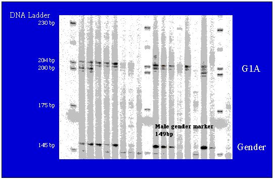
Fig. 8.2. Representative microsatellite and gender probe gel. DNA was amplified by PCR and run out on a Li-Cor
       automated sequencer for scoring by fragment size (number of base pairs).  The individuals are WY black bears.

E. How do we analyze the allelic information?   For a slightly more detailed description go to the Genetic analysis page.
             You can also download my Word document on Web Genetic software.  Luikart and England (1999) provides an (older) overview of approaches.  For use of alternative markers see papers (mostly from TREE) by Sunnucks (2000), Mueller and Wolfenbarger (1999; AFLP), Campbell et al. (2003; AFLP) and Brumfield et al. (2003; SNPs - single nucleotide polymorphisms).

1) Traditional population genetics tools
Heterozygosity (H_obs, H_exp = D)
Hardy-Weinberg equilibrium
Linkage disequilibrium
F_ST and other F-statistics
Genetic distances (Cavalli-Sforza chord, Nei�s 1972 and 1978 distances)
Estimates of 4N_em and 4N_em. (m for mutation, m for migration)


2) Microsatellite specific measures (mostly relying on SMM, Stepwise Mutation Models)

 (delta mu squared) of Goldstein et al. 1995
DSW of Shriver et al. (1995)
R_ST of Slatkin (1995) as implemented by Goodman (1997)
  of Michalakis and Excoffier (1996)
 

3) Newer phylogeographic and population genetic tools
Coalescent inferences (Beerli and Felsenstein, 1999; Rannala and Mountain, 1997)
Assignment tests (Davies et al., 1999; software DOH.html)
Assessment of whether the population is panmictic or shows distinct partitions (Pritchard et al., 2000 and program Structure)
Asymmetric migration analyses (Beerli and Felsenstein, 1999)
Comparisons and contrasts with maternally inherited mitochondrial DNA structure (Piertney et al. 2000; Chesser and Baker 1996).
Assessment of prior bottlenecks.

References:

Beerli, P., and J. Felsenstein. 1999. Maximum likelihood estimation of migration rates and population numbers of two populations using a coalescent approach. Genetics 152: 763-773.
Blouin, M.S. 2003. DNA-based methods for pedigree reconstruction and kinship analysis in natural populations. Trends Ecol. Evol. 18: 503-511.
Brumfield, R.T., P. Beerli, D.A. Nickerson, and S.V. Edwards. 2003. The utility of single nucleotide polymorphisms in inferences of population history. Trends Ecol. Evol. 18: 249-256.
Campbell, D., P. Duchesne, and L. Bernatchez. 2003. AFLP utility for population assignment studies: analytical  investigation and empirical comparison with microsatellites. Mol. Ecol. 12: 1979–1991.
Chesser, R.K., and R.J. Baker. 1996. Effective sizes and dynamics of uniparentally and diparentally inherited genes. Genetics 144: 1225-1235.
Davies, N., F.X. Villablanca, and G.K. Roderick. 1999. Determining the source of individuals: multilocus genotyping in nonequilibrium population genetics. Trends Ecol. Evol. 14: 17-21.
Evett, I.W., and B.S. Weir. 1998. Interpreting DNA Evidence: Statistical Genetics for Forensic Scientists. Sinauer Associates, Sunderland, MA.
Goldstein, D. B., A.R. Linares, L.L. Cavalli-Sforza, and M.W. Feldman. 1995. Genetic absolute dating based on microsatellites and the origin of modern humans. PNAS USA 92: 6723-6727.
Goodman, S.J. 1997. RST Calc: a collection of computer-programs for calculating estimates of genetic differentiation from microsatellite data and determining their significance. Mol. Ecol. 6: 881-885.
Hughes, C.R. 1998. Integrating molecular techniques with field methods in studies of social behavior: a revolution results. Ecology 79: 383-399.
McDonald, D.B., and W.K. Potts. 1997. Microsatellite DNA as a genetic marker at several scales.  pp. 29-49 In Avian Molecular Evolution and Systematics (D. Mindell, ed.). Academic Press, New York.
Michalakis, Y., and L. Excoffier. 1996. A generic estimation of population subdivision using distances between alleles with special reference for microsatellite loci. Genetics 142: 1061-1064.
Mueller, U.G., and L.L. Wolfenbarger. 1999. AFLP genotyping and fingerprinting. Trends Ecol. Evol. 14: 389-394.
Parker, P.G., A.A. Snow, M.D. Schug, G.C. Booton, and P.A. Fuerst. 1998. What molecules can tell us about populations: choosing and using molecular markers. Ecology 79: 361-382.
Piertney, S.B., A.D.C. MacColl, P.J. Bacon, P.A. Racey, X. Lambin, and J.F. Dallas. 2000. Matrilineal genetic structure and female-mediated gene flow in red grouse (Lagopus lagopus scoticus): An analysis using mitochondrial DNA. Evol. 54: 279-289
Pritchard, J.K., M. Stephens, and P. Donnelly. 2000. Inference of population structure using multilocus genotype data. Genetics 155: 945-959.
Rannala, Bruce, and J.L. Mountain. 1997. Detecting immigration by using multilocus genotypes. PNAS 94: 9197-9201.
Selkoe, K.A., and R.J. Toonen. 2006. Microsatellites for ecologists: a practical guide to using and evaluating microsatellite markers.  Ecol. Letters 9: 615-629.
Shoemaker, J.S. et al. 1999. Bayesian statistics in genetics -- a guide for the uninitiated. Trends Genet. 15: 354-358.
Shriver, M.D., L. Jin, E. Boerwinkle, R. Deka, R.E. Ferrell, and R. Chakraborty. 1995. A novel measure of genetic distance for highly polymorphic tandem repeat loci. Mol. Biol. Evol. 12: 914-920.
Slatkin, M. 1995. A measure of population subdivision based on microsatellite allele frequencies. Genetics 139: 457-462.
Strassmann, J.E., Solis, C.R., Peters, J.M., and Queller, D.C. 1996. Strategies for finding and using highly polymorphic DNA microsatellite loci for studies of genetic relatedness and pedigrees. Pp. 163-180In Molecular Zoology: Advances, Strategies and Protocols (J.D. Ferraris, and S.R. Palumbi, eds.). John Wiley and Sons, New York. [See also detailed protocols on pp. 528-549].
Sunnucks, P. 2000. Efficient genetic markers for population biology. Trends Ecol. Evol. 15: 199-203.
Return to top of page