Required readings (PDFs on WyoWeb):

Hudson, P.J., A.P. Dobson, and D. Newborn. 1998. Prevention of population cycles by parasite removal. Science 282: 2256-2258.
Korpimäki, E., and K. Norrdahl. 1998. Ecology 79: 2448-2455.
May, R.M. 1999. Crash tests for real. Nature 398: 371-372.

Return to Main Index page        Go back to notes for Lecture 30,   14-Apr    Go forward to Lecture 32, 19-Apr-13

I will wrap up the section on population regulation with two experimental approaches that serve as useful case histories.  Then I will introduce a brief section on using a clever solution of first-order difference equations to look at disease transmission.  With the recent attention to chronic wasting disease (CWD), sometimes referred to as "mad elk" disease, and the problems related to brucellosis transmission between bison and cattle in Yellowstone, the population ecology of disease spread is clearly relevant.

Predator-prey cycles -- voles and a multi-species assemblage of avian and mammalian predators.

What factors drive the well known population cycles in voles?  From the paper we read earlier by Turchin et al. (2001) we know that the data are consistent with the hypothesis that vole cycle are driven by their predators.  That is, the vole dynamics are like those of prey in predator-prey models (their cycles have blunt peaks).  Korpimäki and Norrdahl (1998) conducted a large-scale experimental reduction of predators.  The voles had four kinds of predators -- least weasels, Mustela nivalis, stoats, M. erminea, Eurasian kestrels, Falco tinnunculus, and Tengmalm's owl, Aegolius funereus.  Their major results were as follows: 1) predator removal did reduce the cycling; 2) it took removal of all the predators to eliminate the cycling -- areas where only one or two of the four predators were reduced still showed prey cycling.

Some questions for you to consider by looking at the Korpimäki and Norrdahl (1998) paper directly

1)  Describe at least two improvements of this study over previous attempts to assess the importance of predator-prey dynamics as a causal factor in rodent population cycles.
2) What factors were important in choosing control areas for comparison to experimental treatment areas?
3) How did the authors assess the pre- and post-treatment densities of the mammalian predators?
4) How did the authors reduce the density of avian predators?
5) What is the importance of the first sentence of the Discussion section of the paper?
6) Reduction of just the least weasel did not prevent the low point in the vole cycle.  What factors do the authors invoke to explain why reduction of all the predators might be necessary to preventing cycling?

Red grouse and parasites. Hudson et al. (1999) studied a classic cyclic population with boom-bust cycles -- the red grouse, Lagopus lagopus (same species that we call Willow Ptarmigan in the U.S.).  The grouse had been broadly acknowledged to undergo density-dependent regulation with time delays.  The key regulating factor, however, was undetermined.  Candidate factors included the food supply (heather and willow), vertebrate predators, parasite infestations, territorial regulation or some other factor.  Hudson et al. discovered that a parasitic nematode (helminthic gut worm) was the likely agent.  Using host-parasite models (more sophisticated versions of the predator-prey models we studied earlier) they made predictions for six populations for which they predicted population lows (of the grouse) in 1989 and 1993.  They conducted an experiment in which they treated populations with antihelminthics (a medicine that kills the gut worms).  Two populations received full treatments before each of the predicted lows.  Two populations were treated only before the 1989 crash.  The last two populations were untreated controls.  The results dramatically  verified the parasite prediction.   The untreated populations crashed to one tenth of one percent of pre-crash population sizes.  One of the two doubly treated treated populations remained steady through the predicted 1989 and 1993 crashes.  The other doubly treated population decreased to a third of its pre-crash size.  One of the two populations treated only in 1989 remained steady in that year but underwent a major crash in 1993.  The remaining population underwent a tenfold reduction in 1989 and a major crash in 1993.  Interestingly, the population with the tenfold crash in 1989 probably received the lowest percentage of bird treatments (approximately 15%).  Host-parasite models suggest a threshold for vaccinations -- only when a certain proportion of the population is vaccinated will epidemics move from cyclic boom-bust outbreaks to lower steady levels.  Hudson et al. estimated that the threshold required to dampen the cycles was approximately 20%.  Again, as in the case of the Isle Royale wolves and moose, the "exception proved the rule".

A commentary on the vole and red grouse papers was the subject of a Nature "News & Views" article called "Crash tests for real" by May (1999).  That should be a useful guide to studying the results from theses two papers.

Bottom line -- focus on nature and strength of interactions among populations.  As suggested by the above example, and the earlier assigned paper by Turchin et al. (2000) on vole and lemming cycles, interactions within and between trophic levels can be complex.  Often, the question may not be one of top-down or bottom-up regulation.  Instead, it may be a matter of the relative strength of interactions (or as in the McQueen pike-bluegill-zooplankton-phytoplankton study, a combination of effects from the top meeting effects from the bottom) .  In some communities, the distribution of interaction strengths may be highly skewed.  A few population links may have very strong interaction effects, while the great majority of interactions between populations are weak.  In those sorts of communities it may be appropriate to talk of keystone species.

Disease is probably a much more important density-dependent regulator of populations than was previously thought.  Recent examples of wildlife diseases that have made the news have been brucellosis (controversial for bison and cattle in the greater Yellowstone area), chronic wasting disease (CWD), with its focus in Colorado and Wyoming, and West Nile virus, which could be much more of a presence in Wyoming this summer.

Many diseases spread in ways that are susceptible to modeling in forms that are somewhat similar to various other models of population dynamics.  We will use a fairly simple difference equation model to make inferences about various population-level aspects of the spread and equilibrium infection rates of an infectious disease.  The model itself was developed in the context of sociology -- to assess the "mobilization" of voters to political parties (the cynical might say that such a process is disease-like).  I adapted this from a formulation in Huckfeldt et al., 1993. As in many of our modeling approaches, we will ignore many complications of the real world in order to focus in on a few key processes that we assume are critical to the process we seek to understand.

Here's the starting equation for the change in the level of infection:

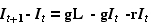                                 Eqn 31.1

where I_t is the proportion of infected individuals at time t,
g is the probability of becoming infected per unit of time (say a year),
L is an upper limit on the proportion of the population that is susceptible, because some individuals are immune (for whatever reason),
and r is the probability of recovering, if infected.
Note that the left hand side (LHS), I_t+1 - I_t , is the same thing as the "change in I_t ."

Rearranging this to be in recurrence form (meaning the value of some variable at time t+1, as a function of the value of that variable at time t) we get

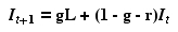                                 Eqn 31.2

[All we did was move I_t to the RHS and factor out all the terms in I_t].

Note that Eqn 31.2 is in the form

Y = b + mX                                                        Eqn 31.3

              {Y-intercept}                              Eqn 31.4

m = (1 - g - r)        {slope}                                   Eqn 31.5

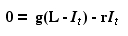                                         Eqn 31.6

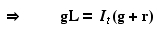                                 Eqn 31.7

                                                  Eqn 31.8

§§§§§§§§§§§§§§§§§§§§§§§§§§§§§§§§§§§§§§§§§§§§§§§§§§§§§§§§§§§§§§§

Return to top of page                                      Go forward to Lecture 32,  19-Apr-13