Return to Main Index page                                      Go to Lecture 35                Go to Lecture 36

N (number of individuals genotyped. The sum of each of the rows in the table above):

Population 1:   500
Population 2:   100
Population 3:   1,000

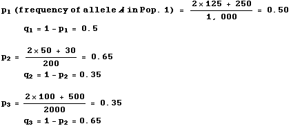
Step 1.  Calculate the gene (allele) frequencies:

Each homozygote will have two alleles, each heterozygote will have one allele.  Note that the denominator will be twice N_i (twice as many alleles as individuals).

              Eqns FST.1

Step 2. Calculate the expected genotypic counts under Hardy-Weinberg Equilibrium, and then calculate the excess or deficiency of homozygotes in each subpopulation.

Pop. 1        Expected AA = 500*0.5²                    = 125     (= observed)

                        Expected Aa =  500*2*0.5*0.5           = 250     (= observed)

                        Expected aa =  500*0.5²                      = 125     (= observed)

Pop. 2        Expected AA = 100*0.65²                   = 42.25  (observed has excess of 7.75)

                        Expected Aa =  100*2*0.65*0.35        =  45.5   (observed has deficit of 15.5)

                        Expected aa =  100*0.35²                      = 12.25  (observed has excess of 7.75)

                     Note that sum of two types of homozygote excess = amount of heterozygote deficiency.
                                    These quantities have to balance (it's a mathematical necessity, given that p + q =1.
 

Pop. 3        Expected AA = 1,000*0.35²                   = 122.5  (observed has deficiency of 22.5)

                        Expected Aa =  1,000*2*0.65*0.35        =  455   (observed has excess of 45)

                        Expected aa =  1,000*0.35²                      = 422.5  (observed has deficiency of 22.5)

Summary of homozygote deficiency or excess relative to HWE:

    Pop. 1.  Observed = Expected: perfect fit
    Pop. 2.  Excess of 15.5 homozygotes: some inbreeding
    Pop. 3.  Deficiency of 45 homozygotes: outbred or experiencing a Wahlund effect (isolate breaking).

Step 3. Calculate the local observed heterozygosities of each subpopulation (we will call them H_{obs s}, where the s subscript refers to the s^th of n populations -- 3 in this example).  Here we count genotypes:

H_{obs 1} = 250 / 500                = 0.5

H_{obs 2} = 30 / 100                               = 0.3

H_{obs 3} = 500 / 1000                                          = 0.5

          Eqns FST.2

(With two alleles it would actually be easier to use 2pq than to use the summation format of Eqn 33.1)

Notation: Note that I am using p₁ and q₁ here (where the subscripts refer to subpopulations 1 through 3).  We would need to use multiple subscripts if we were using the notation of Eqn 35.1 where the alleles are p_i  (and the i refer to alleles 1 to k).  Indeed, with real multi-locus multipopulation data, we would have a triple summation and three subscripts;  one for alleles (i =1 to k), one for the loci ( l =1 to m), and one for subpopulations (s = 1 to n).

          where s (s = 1 to 3) refers to the subpopulation                Eqn FST.3

F₁ = (0.5 — 0.5) / 0.5             = 0

F₂ = (0.455 — 0.3) / 0.455     = 0.341
                                                       [positive F means fewer heterozygotes than expected indicates inbreeding]

F₃ = (0.455 — 0.5) / 0.455     = -0.099
                                                       [negative F means more heterozygotes than expected means excess outbreeding]

Step 6. Calculate     (p-bar, the frequency of allele A) over the total population.

             {genotype splitting method}

or (yields same answer)

              {using Eqn FST.1 values for p_s}

            Note that we weight by population size

Step 7. Calculate  (q-bar, the frequency of allele a) over the total population

Check: p-bar + q-bar =  0.4156 + 0.5844 = 1.0 (as required by Eqn 31.1).

    The check doesn't guarantee that our result is correct, but if they don't sum to one, we know we miscalculated.

Step 8.   Calculate the global heterozygosity indices (over Individuals, Subpopulations and Total population)

Note that the first two calculations employ a weighted average of the values in the whole set of subpopulations.

H_I based on observed heterozygosities in individuals in subpopulations 

                           Eqn FST.4

H_S based on expected heterozygosities in subpopulations

                      Eqn FST.5

H_T based on expected heterozygosities for overall total population (using global allele frequencies and a modified form of Eqn 35.1): 

                              Eqn FST.6

            or we could calculate it as      2*p-bar *q-bar   = 2 * 0.4156 * 0.5844  = 0.4858

Compare and contrast the global F_ISbelow with the "local inbreeding coefficient" F_s of Step 5.
Here we are using a weighted average of the individual heterozygosities over all the subpopulations.
Both F_IS and  F_s are, however, based on the observed heterozygosities,
        whereas F_ST and F_IT are based on expected heterozygosities.

                                             Eqn FST.7

                                               Eqn FST.8

                                             Eqn FST.9

Notation note: the subscripts I, S, and T are not summation subscripts.  They simply indicate the level of our analysis.  Likewise, the s on F_s in Step 5 or on the p_s in Step 1 (the s was implicit there) just tell us what we are referring to.  In contrast, the subscripts for Eqn 35.1 and 35.2 are used in summations and change as we work through the pieces of the calculation.

1)  One of the possible HWE conclusions we could make:

Pop. 1 is consistent with HWE (results of Step 2)

2)  Two of the possible "local inbreeding" conclusions we could make from Step 5:

Pop. 2 is inbred (results of Step 5), and
Pop. 3 may have disassortative mating or be experiencing a Wahlund effect (more heterozygotes than expected).

3)  Conclusion concerning overall degree of genetic differentiation (F_ST)

Subdivision of populations, possibly due to genetic drift,
accounts for approx. 3.4% of the total genetic variation
             (result of Eqn FST.8 F_ST calculation in Step 9),

4)  No excess or deficiency of heterozygotes over the total population (F_IT  is nearly zero).