Lecture 33 (21-Apr-13)
Return to Main Index page Go back to notes for Lecture 32 19-Apr Go forward to Lecture 34 24-Apr-13
The spread of infectious diseases (continued).
Graphical approaches, convergence on equilibrium
Let's continue our analysis of a model for the spread of an infectious disease. In some cases, we may have scattered reports from different places and times that represent the infection level at two successive time intervals. Those data are suitable for plotting and then using as a basis for estimating
the Y-intercept ( b = gL) and
the slope ( m = 1 - g - r),
which then suffice to estimate all the parameters of
interest: ![]() ,
the rate of infection, r, the rate of recovery, L, the upper threshold
of infectability, and I*, the equilibrium level of infection. Let's
say, for example, that we had the data below.
,
the rate of infection, r, the rate of recovery, L, the upper threshold
of infectability, and I*, the equilibrium level of infection. Let's
say, for example, that we had the data below.
{0.200, 0.554}, {0.714, 0.758}, {0.892, 0.623}, {0.817, 0.782}, {0.400, 0.580}, {0.289, 0.622}, {0.598, 0.768}, {0.118, 0.535}, {0.504, 0.621}
Each pair of numbers inside a pair of braces {} represents a sequence of two successive infection levels at times t and t+1: {It, It+1}. We can plot the data as follows:
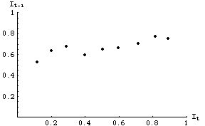
Fig. 33.1. Data for infection levels at time t+1 as a function of infection levels at time t. The different points do not necessarily come from either the same time or place. Each might, for example, represent the successive levels of observed infections in various different states or game management units. All, however, obey the same dynamics (i.e., all have the same underlying values for g, r, and L in Eqn 33.1).
All the points in Fig. 33.1 represent realizations of an underlying linear process modeled by Eqn 33.1. The fact that they do not not line up perfectly along a line (remember Eqn 33.1 is linear) is due to "noise" -- disappearances, emigration or immigration and other factors not included in the model.Eqn 33.1 (= Eqn 32.1= Eqn 31.2)
By using ordinary least squares (OLS) regression we can estimate the Y-intercept, b, and the slope, m. Using Excel, for example, we can use the Chart Option "Add trendline" and the additional option "Display equation" to give us the equation. Doing so would give us a plot something like:
using the equation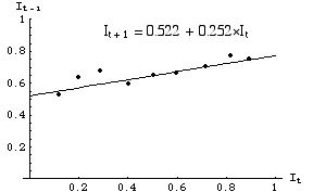
Fig. 33.2. Linear equation fitted to the data points of Fig. 33.1. b = 0.522, m = 0.252. We can now proceed to solve for estimated values of g, r, L and I*.
we can calculate the equilibrium value of infection level. Let's add some lines to Fig. 33.2 to show the equilibrium level.Eqn 33.2 (= Eqn 32.2 = Eqn 31.8)
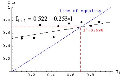
Fig. 33.3. Observed data (points) with fitted linear equation (shallower-sloped solid line), line of equality (blue 1:1 It = It+1), and line for I* (red, dashed line). Note that (by definition) the line of equality crosses the equation line at I*.
The model we have developed will always converge on the equilibrium, I*, eventually. It can, however, approach the equilibrium smoothly or with damped oscillations. Let's begin with the approach exhibited by the data we have analyzed above.
We begin by iterating Eqn 33.1 nine times, starting with a low IØ (e.g., 0.100). Each It+1 then moves to the RHS to become the next It. The result is:
{0, 0.100}, {1, 0.550}, {2, 0.688}, {3, 0.730}, {4, 0.743}, {5, 0.747}, {6, 0.748}, {7, 0.749}, {8, 0.749}, {9, 0.749}If we plot these points we get the following graph:
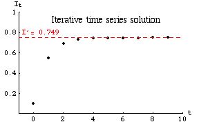
Fig. 33.4. Approach to equilibrium exhibited by iterating Eqn 33.1 from an initial IØ of 0.1. The approach is smooth. Note that the X-axis is in units of t (not the It we have used previously).
Under certain conditions the approach to equilibrium is oscillatory. One way of phrasing those conditions is by saying that the convergence to equilibrium will show damped oscillations when the infection rate (g) is greater than the retention rate (1 - r). This condition can also be stated in terms of the slope of the graph (as you should discover as you complete Homework 7). The graph of the iterative time series solution (data and parameter values not the same as those used for Figs. 33.1 to 33.4) would then be:
§§§§§§§§§§§§§§§§§§§§§§§§§§§§§§§§§§§§§§§§§§§§§§§§§§§§§§§§§§§§§§§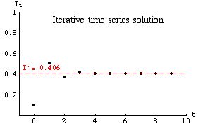
Fig. 33.5. Oscillatory approach to equilibrium [under the condition that g > (1 - r) ] for a linear disease spread model given by Eqn 33.1. Note that the infection level reaches equilibrium on the fourth iteration. Parameter values: g = 0.933, (1 - r) = 0.606.
Question to ponder: What can we say about the slope of the graph of It+1 against It, when we observe oscillatory convergence to I*?