Optional line transect and mark-recapture material
line transect
and mark-recapture methods:
density
estimate from a systematic sampling scheme
Reference:
Burnham, K.P.,
D.R. Anderson, and J. L. Laake. 1980. Estimation of density from line transect
sampling of biological populations. Wildlife Monographs No. 72.
Absolute density? YES.
Count all in study area? NO
Capture or count? COUNT
Is population dense? NO
Can all animals be detected at a distance? NO
How do we deal with incomplete
detectability?
d. Line Transects
Fig. 3.2. Diagram of layout for line transect
sampling scheme. Transect lines are laid out in some systematic fashion
across an area large enough to detect a reasonable sample (>= 40, preferably
more) of "objects" (animals, plants). Observer walks the transect lines
noting distance and angle to objects detected.
Fig. 3.3. Diagram of detection events. Objects
detected have a perpendicular line connecting them to the transect line.
Objects without lines went undetected. Note that objects on the line are
always detected, while those at greater distances have lower probability
of detection. In this example n (number of objects detected) = 13,
including the two objects detected on the transect line itself.
Data that must be collected
for line transect sampling:
Total length of lines traversed, L
(most applications will include replicate lines; these may be parallel
to each other, zigzag in random directions or apply a form of stratified
randomization)
Number of objects detected, n.
Number of individuals within each object (e.g.,
birds per covey)
Perpendicular distance, xi from
transect line to object i (i = 1 to n).
It is usually best also to measure angle and distance from detection point
to object (since many objects will be detected before they are directly
perpendicular to the transect line).
Maximum distance of detection will be w*
(the one-way "width" of the transect detection area). Total "detection"
area will then be 2Lw*.
Sample size (n) of number of objects detected
should be no less than 40.
Rationale (why we need this sort of complex
sampling/counting scheme). The main point here is to overcome the opposite
pitfalls of low accuracy (high bias) on the one hand and low precision
(high variance) on the other, while counting animals in a way that allows
for non-detection of some. That is, in order to get a reasonably high count
of objects detected, we have to accept the fact that we will fail to detect
some objects.
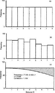
Fig. 3.4. A schematic diagram for
the basic idea behind line transect sampling. You don't need to be
able to read the numbers, just try to grasp the central concept.
The X-axis shows eight distance categories (all objects detected in the
first x meter interval, all objects in the second x meter
interval, etc., where x will be determined by the species being estimated
and the nature of the habitat). The Y-axis shows the percentage
of the total detections represented in each of the given distance intervals.
TOP PANEL. If a population were uniformly
dispersed and we conducted a complete census we should come up with a histogram
of objects at intervals from the center line as shown in the top histogram.
That is, we would fully detect all objects, regardless of distance from
center line � so all the bars in the histogram would be of equal height,
MIDDLE PANEL. In practice, however, detection
will decrease with increasing distance from the center line, as shown in
the middle histogram. These bars are just one particular example
of the general kind of pattern we should expect from actual field data
� we should see a "shoulder" of large bars near the center line, and then
the bars furthest from the center line should be noticeably smaller.
BOTTOM PANEL. The challenge is to estimate
the "undetected" objects shown by the shading in the bottom diagram.
The method of line transect sampling does just that and allows us to compute
an estimate of the total population (shaded plus unshaded portions of the
bottom diagram corresponding to the "full" histogram at the top).
One more point: our estimator is f-hat(0). Think about why that first
bar should be a good basis for going from the middle panel (actual field
detections) to the top panel (hypothetical perfect knowledge).
Our task is to come up with a good estimator
that will allow us to "fill in" the gap between the density (Dw)
of objects we detected (n/2Lw*) and a good estimate of the
actual density. That "fill-in estimator" will be a function we will call
"f-hat(0)", where the hat stands for "estimator".
.gif)
Our end result will be a function to estimate
density given as
 (Eqn 3.1)
In order to get this "fill-in estimator" we need
to make (and meet) some assumptions:
1) Objects directly on the transect line will never
be missed (Probability of detection =1.0)
2)Objects are fixed at the initial sighting position.
That is, they do not avoid the observer before the observer detects them,
and they don�t move away in such a way that the observer risks counting
them twice.
3)Distances and angles are measured without error
4) Sightings are independent events. If we see one
animal it does not affect (positively or negatively) the probability that
we will see other animals.
Examples of violations of these assumptions:
Tropical canopy birds, lizards in rocky terrain, whales
that are submerged as observer�s transect line passes over them
Animal moves prior to detection or double counting occurs
because it moves far enough that observers don�t realize they have already
counted it.
Observers estimate angle and distance poorly
Groups flush
Deriving the basic equations necessary for developing
an estimator.
Let�s start with the most basic equation for population
density. If we had absolutely perfect knowledge, we could write.
D= N/A
(Eqn 3.2)
where D is density, N is population size
and A is area. So say we have 100 animals in a 10-hectare plot (a
hectare is 100 m by 100 m). Then D = 100/10 = 10/ha. When you start
doing equations with mixed units it can sometimes be very important to
keep track of your units. If you had physics think back, for example, to
units of acceleration. Sometimes too, dimensionless numbers are very useful.
In that case, the units cancel.
If we were doing a complete count in a strip transect
of width w, this should be number counted/area covered
 (Eqn 3.3)
where the "hat" over the D means we are
estimating D,
the small n means it is our count (not the full population total
as before), L is the total length of our transects, and w
is the one-sided width of the transect.
Develop a "detection function", which we will call
g(x),
where x is the perpendicular detection distance to objects we detect.
The function g(x) tells us the probability that we will detect
an object, given that it lies a distance x from the centerline of
our transect. What we will do is integrate over the distance from x
= 0 to x = °. This gives us, essentially, the sum of the detection
probabilities.
 (Eqn 3.4)
Now if we divide the original function g(x)
by the integral, a, we will have a function that sums to one (we
have "normalized" it). This function is formally called a probability
density function or pdf.
 (Eqn 3.5)
We have simply rescaled g(x) by
the integral a, to give a function, f(x), that sums
to one [f(x) has exactly the same shape as g(x)!!].
It tells us what the proportion of the total probability is of detecting
an object at a given distance, x occurs at that distance. Say x
= 3.5 meters and the original g(x=3.5) was 0.43. How much
of the total probability (a number that might be much greater than one)
lies at x = 3.5? Again, though the values are different, this new
f(x)
will have exactly the same shape as our original function
g(x).
So, from where we stand on the centerline, we are
asking: what proportion of all the objects out there are we seeing over
the range of distances? At the centerline we assume that we actually see
every
object that is there. Given that we see every object on the line (seems
reasonable) we can say.
g(0) = 1
(Eqn 3.6)
substitute Eqn 3.6 into Eqn 3.5 to get
 (Eqn 3.7)
Now let�s revisit Eqn 3.3.
For a finite w, the probability of detecting an object within the
(half)-strip will be
 (Eqn 3.8)
That is, the total probability, a, divided
by the half-width of the strip, w. If a total of Nw objects
actually occur, the expectation of number of objects we will see will be
E(n) = PwNw
(Eqn 3.9)
where E(n) stands for the "expectation
of n". This is simply the probability of detecting an object
times the total number of objects there. We will know n, the number
of objects we saw, so we can develop an estimator of Nw
as
 (Eqn 3.10)
where we have used the right-hand-side of Eqn
3.8 as a substitute for Pw in the last form of the equation.
Now substitute nw/a for the N of Eqn 3.2
to get:
 (Eqn 3.11)
NOTE that
the w�s cancel out. This means that we can use an "infinite" w
(as far as we can see, or the furthest object detected, called distance
w*).
One more step and we will have our handle on estimating density. Substitute
the left hand of Eqn 3.7 for the 1/a of Eqn 3.11 to get:
(Eqn 3.12 = Eqn 3.1)
Great! If we can just get some estimator f-hat(0),
we can estimate density from our line transect data.
I began by reviewing the derivation involved
in going from Eqn 3.1 back to itself as Eqn 3.12.
Moving from theory and equations to crunching
data and getting an estimate.
I ended last time with Eqn 3.12 (the end result
of deriving Eqn 3.1), which I claimed would be our path to estimating density
from our field transect data. So� our job is to get a good function, f^(0)
for estimating f(0) or its equivalent 1/a.
Real-world issues:
Animals move
Animal response behavior and our ability to detect
them may change during the survey (because of changing wind levels and
other factors.)
Individual animals may respond differently.
Here are the criteria that Burnham and Anderson (1980)
set for a good model of f(x).
General robustness (flexible enough to fit
a range of actual shapes of detection probability).
Robust to pooling (variation in detection
probability factors - some unknown)
Shoulder near zero -- near the centerline
we expect to see almost all the animals (the "shoulder" but then the detection
probability drops off from some moderate distance.
Efficient estimator (low variance, low bias)
The graph below is a histogram of objects detected in
various distance intervals from the center line. It has a "shoulder"
near the center line.
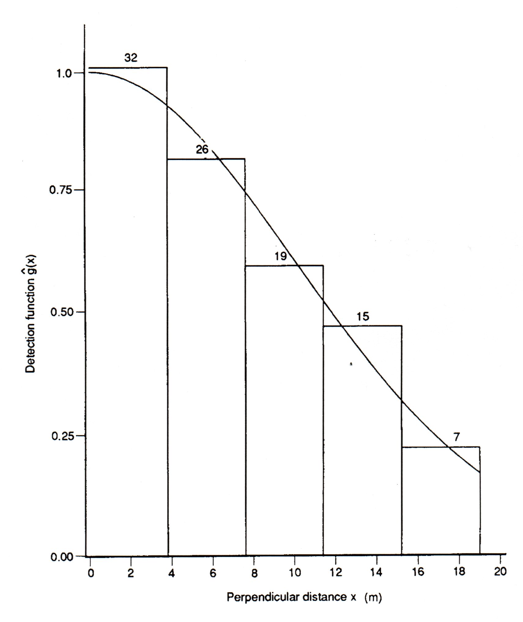
Fig. 3.5. Detection distances (x) for a total
of 99 objects in five distance intervals (3.8 m per interval) from the
transect center line. A detection function g(x) has been
fitted to the observed histogram. Note that the data have been truncated
� 6 objects that were detected at distances > 19 m from the center line
were omitted from the analysis. This truncation makes the analysis
much easier, and more robust, but has little effect on the final estimate
of D. (The truncation means that w* will be 19 meters).
These are the data for the fully worked Excel
spreadsheet example.
Deriving the best estimator goes beyond the scope
of this course. Suffice it to say that sharp minds have shown that a Fourier
series estimator is robust (works under a variety of conditions)
and has reasonable precision and no bias (at least in the limit).
It boils down to an expansion several terms long
that is based on a cosine function of the observed detection distances.
 (Eqn 3.13)
where the w* is just the furthest distance
we actually saw an object at (after throwing out any outliers), the m
is the number of expansion terms (indexed across k). The quantity
a-hat-sub-k is estimated as follows:
 (Eqn 3.14)
So... let�s say we wanted to estimate the term
for k = 1. Start inside the rounded brackets toward the right hand
end. We have 1 (= k) times p,
times xi (our first observed distance; i = 1 to n,
the total number of objects seen), all over our maximum distance, w*;
take the cosine of that. Now comes our summation term. Work through our
full set of distances (i = 1 to
n) and add all those n
terms together. Multiply that sum of n terms by 2/nw*. That�s
a-hat-sub-k.
Even better, a computer program can do it all for us.
Note for calculations from
"heaped" data (like the homework problem and LineTransect.XL). The
above formula works best when each of the sighting distances is recorded
separately (the actual measurement) rather than when working with midpoint
distances for lumped data.
For lumped data we can rewrite Eqn 3.14 as follows
so that the calculation method is more explicit:
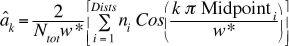 (Eqn 3.14a)
here we see explicitly the term Ntot for ALL the objects
detected versus the ni (number of objects detected in
distance category i, where i goes from 1 to Dists,
the number of "lumps" or distance categories � 5 in the example in LineTransects.XL
and 6 in your homework problems). Rather than go one by one through
all the objects we do the Cosine operation on each of the Midpointi
distances TIMES the number of objects, ni , in that lump
(at that midpoint distance).
CALCULATORS: RADIANS vs. DEGREES.
Excel and some calculators assume the input is in radians, as do the formulas
above. However, your calculator may use degrees instead. In
that case, you would want to use the term:
Cos[ (k 180 Midpointi)/
w*]. That is, you would need to multiply the stuff inside the cosine
bracket by 180/p
before taking the cosine. (Since p
was already in the denominator it cancels out).
Alternatively, you may be able to set
your calculator to work in radians. Here's how to check which of
the two your calculator is doing. Take the cosine of 1.0. If
your answer is 0.5403 then you are working in radians and everything is
fine. If your answer is 0.9998 then you are working in degrees. You
must either convert values to radians by multiplying by 180/ or switch
your calculator to do its calculations in radians.
I have run fairly quickly through sets of equations
related to line transect sampling. Let�s look back at the high points.
First I used various equations related to density to
show that
(= Eqn 3.1 = Eqn 3.12)
I then said that if we could just estimate f(0)
we could turn that back into an estimate of density, given the observed
number of animals, n., and our transect length, L. The estimator
function we will use is based on a Fourier series:
 (Eqn 3.15 = Eqns 3.13 + 3.14)
Here is a summary of the real-world issues:
Animals move
Animal response behavior and our ability to detect them
may change during the survey (wind level etc.)
Individual animals may respond differently.
Here are the criteria that Burnham and Anderson
set for a good model of f(x).
General robustness (flexible enough to fit
a range of actual shapes of detection probability).
Robust to pooling (variation in detection probability
factors - some unknown)
Shoulder near zero
Efficient estimator (low variance, low bias)
That ROBUST estimator is the Fourier series function
given in Eqns 3.13 and 3.15.
We had a question about the stopping rule for the number
of terms in the theoretically infinite number of terms in the Fourier series
expansion. That rule is to use the first value of m that fits the
following criterion:
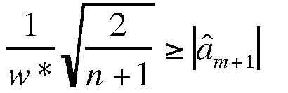 (Eqn 3.16)
That is, we look one step ahead (at m+1) and
see whether the inequality is met. If so, then we use m; otherwise,
we proceed to try m+2. For the
interested: that stopping rule is based on a principle called MISE (minimum
integrated
squared
error;
it is not something I expect you to remember).
(Eqn 3.16)
That is, we look one step ahead (at m+1) and
see whether the inequality is met. If so, then we use m; otherwise,
we proceed to try m+2. For the
interested: that stopping rule is based on a principle called MISE (minimum
integrated
squared
error;
it is not something I expect you to remember).
We�ve now covered some of the the theory of line
transect sampling and obtained an idea of how we can turn field data in
actually calculating a density estimate. We�ll now turn to a brief consideration
of possible layouts for the transects. You may remember that I mentioned
that one will usually want multiple transect lines that sum to L.
Mathematically
 (Eqn 3.17)
That is, we will have q transects whose total
summed length is L.
(Eqn 3.17)
That is, we will have q transects whose total
summed length is L.
Here are two possible schemes. Which is the more
practical? Which is the "ideal"?
Fig. 3.6. Transect lines (l1
to l7; ·li = L) selected
with random starting points and common (but randomly selected) direction.
Lines may be of equal or unequal length.
Fig. 3.7. Transect lines (l1
to l8; ·li = L) each
selected with a random starting point and a randomly selected direction.
Lines are of unequal length.
The bottom case is arguably the ideal, because each
of the lines has a randomly selected direction and length. In practice,
this sort of design will be exceedingly difficult to carry out, so we might
go with the upper case. Even that may not be possible so we may need to
go with one of the following.
We could use any of a series of different possible
layouts. These could include connected lines with "kinks" that change angle,
systematic designs that cover the study area in a regular design, or subdivided
plots that partition the study area.
Somehow, though, we should try hard to incorporate
some randomization. This could involve
a randomly selected starting point on the perimeter, a randomly chosen
angle for the parallel transect lines, or some other way of avoiding systematic
bias (again, at all costs we want to avoid some obvious source of bias
such as paralleling ridge tops.
SUMMARY of considerations in designing the layout:
Define the population of interest
Delimit the population (figure out the logical and
logistically feasible boundaries)
Devise a sampling scheme that truly samples the population
of interest
Conduct a survey the gathers the required data
Goal of the design: Sample the population of interest
in a way that yields an adequate representation of reality
To meet the goal in practice:
Every member of the population must have an equal
probability of being sampled
(can�t have submerged whales that are not susceptible
to sighting)
Must have adequate replication (adequate
sample size)
Sample must have adequate spatial dispersion
(and possibly temporal dispersion)
Must avoid correlation between transect orientation
and particular features of the landscape (such as ridges or valleys).
It�s acceptable to have one line (of many) that (by chance) aligns with
the environmental feature (road, river), just not that they ALL do so --
that may produce bias.
Must bring randomization into the design process
at some point -- the more the better, but if nothing else then a random
starting point or random direction (for parallel or systematic designs).
See the Excel
spreadsheet (link below) for a fully worked example of applying the Fourier
series estimator and the stopping rule to the set of data given in Fig.
3.5.
Go
to Excel spreadsheet
Here is a website for the current documentation
on line transect sampling using the program DISTANCE
http://www.colostate.edu/depts/coopunit/distancebook/download.html
Burnham and
Anderson Distance manual for software (including line transect analysis)
in pdf format
End of material on line transect
sampling
________________________________________________________________________
Our next topic will be
mark-recapture
schemes.
The simplest scheme here is the Lincoln-Petersen index.
Note that it is not really an index but an estimate. Refer back to the
dichotomous
key of estimation techniques in Lecture 8 to see where
it falls. We have four variables, three of which we will be able to measure
-- we can solve one equation in one unknown.
N = population size (we won�t know
that, normally)
M = initial sample that we mark
n = number recaptured
m = number in recaps that are already marked.
Here�s the (low bias) formula for the estimated population
size:
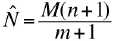 (Eqn 3.18)
The variance of this estimate is given by the following
formula:
(Eqn 3.18)
The variance of this estimate is given by the following
formula:
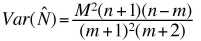 (Eqn 3.19)
From the variance, we can calculate a confidence interval.
The confidence interval (abbreviated CI) tells us the limits between which
we are 95% sure the true estimate lies. The most common alpha level is
0.05 (leading to a 95% interval) but we could use alpha = 0.10 (leading
to 90% CI) or alpha = 0.025 (leading to 97.5% CI). The formula is:
(Eqn 3.19)
From the variance, we can calculate a confidence interval.
The confidence interval (abbreviated CI) tells us the limits between which
we are 95% sure the true estimate lies. The most common alpha level is
0.05 (leading to a 95% interval) but we could use alpha = 0.10 (leading
to 90% CI) or alpha = 0.025 (leading to 97.5% CI). The formula is:
 (Eqn 3.20)
where the upper CI is our original estimate plus
the term on the right and the lower CI is the original estimate minus
the term on the right. The t refers to a value taken from Student�s
t-distribution
and will depend on our sample size (determining the degrees of freedom
abbreviated d.f.) and the alpha value. For a sample with a large
degrees of freedom (>30) and an alpha of 0.05, the t-value will
be approximately 2. That means that our CI will be the original estimate
plus or minus two standard deviations (s.d. = square root of the
variance).
(Eqn 3.20)
where the upper CI is our original estimate plus
the term on the right and the lower CI is the original estimate minus
the term on the right. The t refers to a value taken from Student�s
t-distribution
and will depend on our sample size (determining the degrees of freedom
abbreviated d.f.) and the alpha value. For a sample with a large
degrees of freedom (>30) and an alpha of 0.05, the t-value will
be approximately 2. That means that our CI will be the original estimate
plus or minus two standard deviations (s.d. = square root of the
variance).
Last time we began on mark-recapture schemes. Remember
to look back at where it lies on our dichotomous key. Unlike line transect
sampling, which is largely restricted to obtaining a density estimate,
mark-recapture can actually do several things for us. It can help us estimate
one or more of the following:
Type A (can focus just on marked animals)
Movement of individuals
Growth rate (size/weight) of individuals
Age-specific fertility rates
Age-specific survival rates
Type B (requires estimation of proportion unmarked)
Size of the population
Birth + immigration
Death + emigration
Rate of harvesting
The first four "outputs" require only that we be able
to identify marked animals. We can ignore the unmarked individuals. For
all of the Type A and Type B methods, though, we are assuming
that loss of marks either doesn�t occur or is negligible.
One way to test that assumption is by a double-banding
study. Then we have four kinds of animals
Those with both bands
Those with one band (lost one)
Those that lost both bands
Those that were never marked.
We can identify only those animals in the first two
categories. Nevertheless, the data allow us to generate expectations of
proportion with one or two bands. If our data differ significantly from
the predicted values, then we have reason to suspect that band loss is
biasing our results.
To use mark-recapture for estimating density and
the other Type B uses, we are interested in both the caught and the uncaught.
In that case we have one overriding assumption that we should meet
Equal catchability for all.
Why might we fail to meet that assumption?
Individuals may differ inherently in their behavior
at traps or marking stations
Individuals may learn to seek or avoid traps
or marking stations
Spatial dispersion may affect opportunity for
capture (can�t catch an animal if the trap is not in its home range)
The last assumption can be addressed by proper
randomization. Even with randomization, sexes may differ in catchability
(home range size) and may need to be analyzed separately.
The second assumption can be tested by analysis of
the pattern of captures and recaptures.
The simplest scheme here is the Lincoln-Petersen index
(or Petersen estimate). Again, the parameters we need for this are:
N = population size
M = initial sample that we mark
n = number recaptured
m = number of recaptured individuals (n) that are already
marked.
We start from the premise that the ratio of the population
to the marked will equal the ratio of our first capture (n) to the number
already marked caught in the second round.
 (Eqn 3.21)
Unfortunately, that simplest estimator has been shown
to be biased. Two estimators exist that work on the bias. The following
formula has low bias:
(Eqn 3.22 = 3.18)
from which we can calculate a variance given by:
(Eqn 3.23 = 3.19)
we can then generate a confidence interval for the population
size estimate by using
(Eqn 3.24 = 3.20)
for example we might be seeking to say that we are 95%
confident our estimate lies between upper limit 1 and lower limit 2.
(Eqn 3.21)
Unfortunately, that simplest estimator has been shown
to be biased. Two estimators exist that work on the bias. The following
formula has low bias:
(Eqn 3.22 = 3.18)
from which we can calculate a variance given by:
(Eqn 3.23 = 3.19)
we can then generate a confidence interval for the population
size estimate by using
(Eqn 3.24 = 3.20)
for example we might be seeking to say that we are 95%
confident our estimate lies between upper limit 1 and lower limit 2.
Last time I gave formulae (Eqns 3.22 to 3.24) for
reduced bias estimation of the population size, its variance and a confidence
interval. We can use Eqn 3.24/3.20 to calculate a confidence interval on
our estimate. The attached Excel spreadsheet provides a concrete example
of all the necessary calculations.
Go
to Mark-recapture Excel spreadsheet
Say we caught and marked 301 animals on a first round
and captured 236 on a second round. If 146 of the animals were previously
marked our  would be
485, the variance would be 604.3 and the 95% CI would range from 437 to
534 (= ± 10 % of ).
would be
485, the variance would be 604.3 and the 95% CI would range from 437 to
534 (= ± 10 % of ).
[That CI corresponds to an alpha level of 0.05 and
we use a Student�s t-distribution with the requisite number of degrees
of freedom to calculate the interval].
The estimator above is still somewhat biased. We
can come up with a completely unbiased estimator by deciding beforehand
on a number of recaptures (m). We continue trapping until we catch
the required number of already-marked individuals. In that case our estimate
is:
 (Eqn 3.25)
and the corresponding variance estimate is:
(Eqn 3.25)
and the corresponding variance estimate is:
 (Eqn 3.26)
We can use Eqn 3.26 to figure out how many animals we
need to mark (M) and then recapture (m) in order to get a
standard deviation for N-hat that is acceptable. Say we want to
get a s.d. of <10% of .
For a total population size (N) between 100 and 1000 we then need
the following numbers of M and m.
M {100, 200, 250}
(Eqn 3.26)
We can use Eqn 3.26 to figure out how many animals we
need to mark (M) and then recapture (m) in order to get a
standard deviation for N-hat that is acceptable. Say we want to
get a s.d. of <10% of .
For a total population size (N) between 100 and 1000 we then need
the following numbers of M and m.
M {100, 200, 250}
m { 55, 80, 90}
Using our previous example: if we captured and marked
301 (=M) animals on the first round, then set a goal of 151 already
marked (= m). Say it takes us 244 captures to reach that goal.
=
491, Var () = 612.9, 95%
CI = 442 to 540 (= ±
9.96%).
Notice that in the two previous examples we caught
a fairly large percentage of the total population (in fact 40-60%). It
may not always be feasible to catch that high a proportion of the population.
In that case we can use the slightly more complex multi-capture method.
We can use methods developed by Schnabel in the 1930's and modified by
Schumacher and Eschmeyer in the 1940's. The applications were developed
largely for estimating fish populations. (Method 4
of our dichotomous key)
 (Eqn 3.27)
In the 1960�s G.M. Jolly and G.A.F. Seber began modifying
these multi-capture techniques in various ways that allowed them to serve
both Type A and Type B estimation purposes. These multi-capture methods
have been the subject of intensive analysis since then, and are the basis
for numerous software programs that analyze survival (I�ll come back to
the software programs in a later lecture). I�m not going to take the time
to go into those but extensive references exist for using such methods,
including Caughley�s book Analysis of Vertebrate Populations. Look back
at where the different options lie on our dichotomous
key. Depending on whether we are more interested in knowing
about survival rates or are still more interested in estimating abundance,
we will wind up at methods 10,
11
or 13 of the key
(what does that mean about a fundamental population
assumption early in the key?).
(Eqn 3.27)
In the 1960�s G.M. Jolly and G.A.F. Seber began modifying
these multi-capture techniques in various ways that allowed them to serve
both Type A and Type B estimation purposes. These multi-capture methods
have been the subject of intensive analysis since then, and are the basis
for numerous software programs that analyze survival (I�ll come back to
the software programs in a later lecture). I�m not going to take the time
to go into those but extensive references exist for using such methods,
including Caughley�s book Analysis of Vertebrate Populations. Look back
at where the different options lie on our dichotomous
key. Depending on whether we are more interested in knowing
about survival rates or are still more interested in estimating abundance,
we will wind up at methods 10,
11
or 13 of the key
(what does that mean about a fundamental population
assumption early in the key?).
References for
the interested:
Caughley, G.
1977. Analysis of Vertebrate Populations. Wiley, New York.
Jolly, G.M. 1965.
Explicit estimates from capture-recapture data with both death and immigration
-- stochastic model. Biometrika 52: 225-247.
Schnabel, Z.E.
1938. The estimation of total fish in a lake. Am. Math. Mon. 348-352.
Schumacher, F.X.,
and R.W. Eschmeyer. 1943. The estimation of fish populations in lakes and
ponds. J. Tenn. Acad. Sci. 18: 228-249.
Seber, G.A.F.
1965. A note on the multiple capture-recapture census. Biometrika 52: 249-259.
Some web-based resources
for analysis of populations:
http://www.stanford.edu/group/CCB/Eco/popest2.htm
Stanford U.
population
estimation page
http://canuck.dnr.cornell.edu/misc/cmr/
Evan Cooch
(Cornell) page of mark-recapture software and sources
http://www.cnr.colostate.edu/~gwhite/mark/mark.htm
Gary White
(CSU) page of software etc.
Interestingly, the Jolly-Seber method is more widely
used for our next topic -- estimating survival or mortality rates. Much
of the analysis of survival in natural populations is based on marking
animals and then using the patterns of recapture to make inferences about
survival rates. Obviously when we start focusing on survival rates we
can�t be talking about a closed population.
We will start next time with an overview of patterns
of mortality.
END of line transect and mark-recapture
§§§§§§§§§§§§§§§§§§§§§§§§§§§§§§§§§§§§§§§§§§§§§§§§§§§§§§§§§§§§§§§
Return to top
of page