Logistic growth, lags, patterns of variation in the growth rate (l or r)
and more on the equation for logistic growth.

Return to Main Index page       Go back to notes for Lecture 4,  23-Jan     Go forward to notes for Lecture 6,  28-Jan

Last time I discussed one of the simplest models for population growth -- exponential.  Do  populations ever grow exponentially?  Yes, under some circumstances (and for finite periods of time). For most of today's lecture, I will discuss a model that is slightly more realistic (in most cases).  I will present some of the ways in which populations can oscillate (violating an assumption of our first few simple models), some of the factors that can affect the growth rate (r or l), and then come back to the logistic equation and some of its mathematical properties.

First, though, let's consider under what conditions populations do grow exponentially:

1) Invasive species when they first arrive (New Zealand mud snails in the Yellowstone ecosystem)

2) Species colonizing a new habitat (e.g., an isolated island)

3) Species that are rebounding from a population crash (black-footed ferrets in the Shirley Basin, WY)

4) When they develop novel adaptations to cope with the environment (does a familiar species spring to mind?)

[Note that the first part of logistic growth (the sigmoid curve up to the inflection point) is essentially exponential growth]

Do populations normally grow exponentially? Why not?

        Adding (a little ) realism

In most cases, if we model curves like those in Fig. 4.1 (previous lecture) in the light of real world populations, we can tell immediately that something is wrong.

If a model gives an obviously wrong answer, CHECK THE ASSUMPTIONS.

The hidden (and patently false) assumption here is that the birth and death rates are constant -- that is, we implicitly assumed that the birth and death rates were independent of the population size and wouldn't change over time.
I presume all of you know the simplest way to correct the graph and the name of the corresponding equation.
Right… the logistic. Let's look at a graph of logistic population growth:

Figure 5.1. Logistic population growth -- the plot shows population size (N) as a 
function of time (t).  At first, the population grows essentially exponentially.
At a population size of K/2 the growth rate begins to decline and eventually reaches an
asymptote at the carrying capacity, K. The "braking agent" is the additional term
(K-N)/K -- try various values of K and N to see what effect the term will have on exponential growth. Some of what the course will do is explore the factors that influence or determine K.  Note that the form of the "solution" (to the right of the curve) is in a different form/rearrangement than in Eqn 5.2.  Note also that the familiar sigmoid curve is NOT a plot of  the logistic equation (Eqn 5.1) but of its solution (Eqn 5.2).

• 1) What happens when N> K?
• 2) At what point is the population growing most rapidly? How would you find that mathematically?
• 3) What are the stability/equilibrium characteristics of the logistic compared to the exponential?
        Do we have a new one, in addition to N = 0 and r = 0?
• 4) How would you interpret the first and second derivatives of the equation to the right of the curve in Fig. 5.1?
            Is either of those related to the equation on the left of the curve?
• 5) If this were a harvested population, where would you like to maintain the population size in order to manage
        for Maximum Sustained Yield (MSY)? Optimum Sustained Yield (OSY)?

Hidden assumptions:

1) Environment is constant except for crowding effect
        (e.g., no stochastic effects of weather, no disease epidemics)

2) Effects of crowding are age-independent
        (whereas in fact, density-dependence tends to have strongest effects
            on juveniles and post-prime)

3) No effect of time lags
        (as we'll see later in the course, time lags can have dramatic destabilizing effects).

One obvious example of violations of assumptions 1) and 3) is deer irruptions: the population greatly overshoots the carrying capacity (response to crowding therefore lags behind the equilibrium zero growth point). This damages the habitat (possibly irreversibly and definitely on a time scale of several generations of the herbivore) and changes the environment. Let's graph that, along with some other variations on the theme of logistic growth.

Fig. 5.2. A population irruption in which the population "overshoots" the carrying capacity, K, and then crashes precipitously. Note that after the crash the population rebounds somewhat and approaches a new stable size (dN/dt = 0). Note that the carrying capacity has also changed. In the case of the Kaibab deer, this would represent irreversible (or at least very long term) changes in the amount of food available.

Fig. 5.3. A population showing damped oscillations. At first it overshoots K fairly substantially but then instead of crashing, it dips below the line and back over until finally settling at the asymptotic size, K. This pattern of damped oscillations might occur after some introductions. At first the populations responds rapidly to a vacant niche, but eventually settles to a reasonably steady equilibrium size.

Fig. 5.4. A population showing undamped oscillations. It first overshoots K then dips below the line and back up without ever settling at the asymptotic size, K. This pattern of undamped oscillations characterizes some voles, snowshoe hares and other species that tend to exhibit population cycles.  

Think of a combination of water temperature and current velocity affecting a trout population. We might get a "topographical" plot approximately like this:

Fig. 5.5. Combined effects of water temperature and velocity of stream current on the population growth rate of a hypothetical trout population (in the absence of other factors such as interspecific competition).  Here, the conditions vary in a smooth clinal way -- best at the center and gradually getting worse as we move away toward higher or lower temperatures (X-axis) or higher or lower current velocities (Y-axis).

In some cases, suitability may vary more patchily in space.  Some patches may be "suitable" (l >= 1) while other areas are unsuitable (l< 1 or even essentially 0).  In the graph below I have made some of the patches "sources" (l > 1), some "sinks" (l < 1, but not near zero) and much of the habitat simply unsuitable (l essentially 0).  [A "sink" is an area where the local population declines.  Individuals that disperse into that area will be effectively "going down the drain." A "source" is an area that produces an excess of individuals some of whom can then disperse to other areas]. 

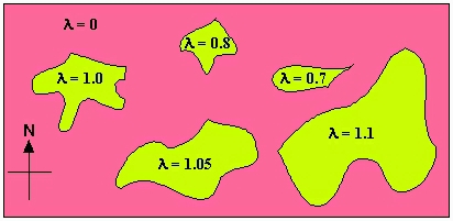
Fig. 5.6. Map of variation of l as a function of spatial variation (e.g., suitable boulder piles for shelter, or meadows for food and burrows, or forest for three-dimensional structure).  Pink denotes completely unsuitable habitat, while the greenish yellow denotes areas of varying suitability.  Spots of high suitability (l > 1) serve as "sources" from which other patches can get subsidies.  These poorer patches act as "sinks" (with l< 1) .  In this case, the pattern of l values suggests that patch area may be an important source of variation in suitability (one possible experimental test would be to decrease the size of some patches and increase that of others to see whether the l values change accordingly).  This sort of source-sink dynamic is the subject of much of the theory of metapopulations. [See: Pulliam, H.R. 1988. Sources, sinks, and population regulation. Am. Nat 132: 652-661]

The logistic equation uses exponential growth as its base, but then adds a "braking force" as numbers increase toward the "carrying capacity", K. The equation is:

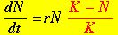                                         (Eqn 5.1)

The portion in black is the exponential growth equation (Eqn 4.6). The new term (in red) discounts exponential growth by the difference from the carrying capacity. For a small population the term in red is near 1.0 and growth is essentially exponential. As the population, N, nears K, growth slows (and can be negative for N > K).  This is a continuous, differential equation.  Later in the course we will deal with a discrete (difference equation) form of the logistic (which can have very different dynamics).  We will revisit continuous logistic growth when we consider models of competition and predation.

Point to ponder: We have a new stable point -- what is it, and what is its "domain" (that is, is it neutrally stable, locally stable or globally stable)?

One can solve Eqn 5.1 using the same technique as in Eqns 4.6 to 4.12. [Try doing this]. The result is:

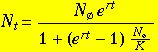                                      (Eqn 5.2)

Eqn 5.2 is what one actually plots in order to obtain the familiar sigmoid curve of Fig. 5.1. Changing the value of r will affect the steepness of the ascending portion. Note that there are several ways to express the right-hand side of Eqn 5.2. I prefer some variant of the form above because it has one part (the numerator) that clearly relates to the solution of the exponential growth equation (Eqn 4.12). The other part (the denominator) is the "braking force".

Study hint:  When I refer to an equation or figure from a previous lecture, try recreating it without looking back at it.  Then open the web page (you can do two at once) or the page in the printed notes, and have it there for reference.

Logarithms and linearity. One of the properties of the exponential growth we plotted earlier is that a semi-log plot will be linear . That is, if we plot the natural logarithm of population size against time, the plot will be linear.

Fig. 5.7.  (Nonlinear) plot of exponential growth, with X-axis as time and Y-axis as population size (same as Fig. 4.1).

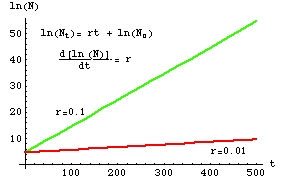
Fig. 5.8.  Log-linear transformation of the exponential growth plot in Fig. 5.7.  Note that the slope of the "curves" is now just r (verify this by using the linear equation format shown in Eqn 5.3).

The logistic equation can also be linearized -- the log-linear form is more complex than the one shown for the exponential equation in Fig. 5.8, but the principle is the same (you will work with this feature in a future homework). Here's a specially rearranged (we'll see why shortly) linear transformation of the logistic equation:

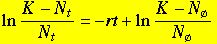                                          (Eqn 5.3)

Eqn 5.3 is of the form for a basic linear equation:

Y = mX + b                                                                             (Eqn 5.4)

where m is the slope, and b is the Y-intercept, of a linear regression of Y against X.  For our population equation (Eqn 5.3), the X-axis will be time (t), while the Y-axis will be the left-hand side (LHS) of Eqn 5.3.  The main utility of Eqn 5.3 is that the slope of the plot of the equation is -r. Now let's see how we use that to solve for r from real-world data on observed population sizes over time.

Note on notation:  in lecture and these web notes, I will often refer to the left-hand side of an equation as the LHS and to the right-hand side as the RHS.

Estimating the r from real-world plots of N against time, when growth is logistic. The problem with equation 5.3 is that we have one equation with two unknowns (K and r).  How can we find their values?

With an observed set of measurements of population size against time, we can estimate r by plotting the untransformed data (with X-axis, t and Y-axis, population sizes at various times t) and then:

1)  eyeballing an estimate of K (the asymptote or place where the curve flattens out)

2)  since we now have an estimate of K (and already knew N_Ø and N_t), we can solve Eqn 5.3 for r

3)  or, we can estimate r graphically, as (the negative of ) the slope of the plot of Eqn 5.3.

Return to top of page           Go forward to notes for Lecture 6,  28-Jan