(Eqn 4.1)
Lecture notes for ZOO 4400/5400 Population Ecology
Lecture 4 (23-Jan-13)
How to learn;
Inflow, outflow, introduction to exponential growth.
Required reading: Gotelli text, Chapter 1 and Appendix (in "Required Readings" folder on WyoWeb;
Krebs, Instantaneous and finite rates (in "Handouts" folder on WyoWeb)
Suggested reading: Wilson and Bossert, Chapter 3 -- Ecology (on WyoWeb in "Suggested readings folder")
Return to Main Index page Go back to notes for Lecture 3, 18-Jan Go forward to notes for Lecture 5, 25-Jan
Last time I discussed the value of mathematical models and experimental approaches (something we will come back to from time to time throughout the course), and quickly considered the characteristics of pseudoscience.
Before I turn to models of exponential and logistic growth, I want to offer some thoughts on the learning process. How to learn: It's up to you. "One of the most discouraging features about teaching is the widespread conviction among students that the process of learning is something bequeathed by the teacher, by a book, or by TV to the student. It is a startling revelation to many that learning is an active endogenous process, that learning is done by the individual by himself." (Vincent Dethier, author of To Know a Fly). Put differently, the quotation above suggests that my job is not to teach, but to facilitate your learning. Students sometimes think that if they recognize material they "know" it. For better or worse, learning is harder than that. You haven't learned something until you can use it yourself, possibly in a context rather different from the one in which it was presented to you. That's why exam questions in a course like this one may seem not to have "been in the notes". You will NOT succeed in this course if all you know is rote memory of the material in the lectures and readings. You must learn to see the material from a variety of angles. Learn by doing. Practice: Try out the logic of the arguments. See whether you can reconstruct the chain of thought without having to refer constantly to your notes or the readings. Set up graphs and label the axes without looking back at your notes or the text. Compare and contrast the methods and assumptions of different approaches to the same problem or the same approach to different problems. For modeling and the application of mathematics to ecology and evolution, the more you do it, the better you do it and (believe it or not) the easier it becomes. Reading over the lecture notes before each lecture should also really help it fit into context.
Some of what we learn this semester will eventually be out of date -- most of it, however, consists of very general principles (and some mathematical and graphical tools) that are essential starting points for any exploration of new approaches. Furthermore, some workers do things that still apply and that can stimulate new approaches and discoveries far into the future (Darwin's insights, the British mathematician G.H. Hardy's insights into elementary population genetics, Maynard Smith's introduction of game theory and ESS (evolutionary stable strategy) approaches, Aldo Leopard's syntheses). The lectures and tests will sometimes highlight disagreements among scientists regarding particular concepts. This may disturb you ("What's the real answer?!?"). Arguments and controversies DON'T mean that anyone's guess is as good as anyone else's. They do mean that the subject area is in an exciting stage -- in which it is important to set up clear alternatives and debate them so that the final picture is sharper. A classic example of a big battle was that between Andrewartha and Birch (favoring density independent regulation) and Lack (favoring density-dependent regulation). What you'll learn, I hope, is that they were both right, and both wrong. Much hinges on the context (Lack studied birds, Andrewartha insects) and the temporal and spatial scale is very important. The debate forced everyone to sharpen their logic, and provided the basis for a huge array of conceptual advances, hypotheses, models, observations and experiments all of which contributed to solid progress in understanding. One could look at this "conflict" as a sort of intellectual natural selection. Only if several alternatives exist can a hypothesis be subjected to the kinds of critical scrutiny and evaluation that makes for a robust theory or law.
How do populations change in size? Four major processes are at work:
B
D
I E
(symbols used in Eqn 4.1)
Birth, death, immigration and emigration.
+
-
+
-
We will start simple, and
ignore
immigration and emigration for the moment. So now we are looking at
birth
and death rates. At the very simplest level, if the births outweigh the
deaths we have a growing population, if the deaths predominate, the
population
shrinks.
Right away we face a
choice:
should we delve
into the complexity of different life cycles,
getting the data in the field and how to tally the births and deaths
or
should we build
a framework of the mathematical approaches that provide a conceptual
basis for understanding? The Gotelli Primer chooses
the latter. I will go with the latter -- we will set up some very basic equations
and then see how we should fit real animals or plants and real world data
into them later. As a complement to the lectures I suggest reading Chapter 1
of Gotelli and peeking ahead at his Chapter 2, I have also put some
excerpts from the classic "Primer of Population Biology" of Wilson
and Bossert on WyoWeb. The Chapter 1 excerpt is
part of the required reading list (it was the source for much of the material
that follows in this lecture). If you plan to stay in biology/ecology
I strongly recommend you buy the book. We start with one of the
simplest kinds of population growth -- exponential. An interest in the
ability of populations to grow rapidly goes back at least to Leonardo Fibonacci
in 1202 (800 years ago!), who considered the problem of unchecked breeding
by rabbits. In 1798 the Reverend Thomas Malthus published "An Essay
on the Principles of Population Growth as It Affects the Future Improvement
of Society". This was the book that played a key role in Darwin's
formulation of the principle of Natural Selection. Gotelli or someone
said that the heart of population ecology is to understand the factors
that keep most populations
from increasing exponentially most
of the time. These factors that keep populations in check
include intra- and inter-specific competition, predation, a harsh environment and
disease. Together or separately they REGULATE populations, so that most
populations neither explode nor crash. Much of what we will do in
this course is to explore the ways that populations persist -- and figure
out how and why they don't persist everywhere and forever.
We'll begin with a continuous, differential equation with four kinds of inflow and outflow:
where B is number of births, I is number of immigrants, D is number of deaths and E is number of emigrants. This equation is what's called a differential equation. It is expressed as a derivative (where dN/dt means the change in N with a change in t). Change (usually change in time), will occur continuously. Working with differential equations often requires us to use the techniques of differential calculus.
The alternative is to use difference equations -- with that technique, time changes discretely (time changing by integer increments such as first year, second year etc.). An example of a difference equation for population growth is Nt = 1.1* Nt-1
In Eqn 4.1, the population size can change via movement (exogenous -- meaning generated outside -- inflow and outflow from/to other populations) as well as via reproduction/death (endogenous -- meaning generated inside -- flows occurring within the population). For the time being, though, we'll ignore movement (I and E; an example of simplification and abstraction), so we're left with:
(Eqn 4.2)
Now, let's think about the numbers B and D. It seems reasonable to suppose that they will depend on population size. That is, a large population will have both more births and more deaths than will a small population. Mathematically we could phrase this as:
(Eqn 4.3)
the little b and little d now refer to the death RATE per individual rather than the total number of births or deaths. For two populations of different size, but with the same birth and death rates, the size of B or D then depends on N, the population size. For example, we might have the same birth and death rates (1 calf per female per year) and death rates (30% mortality per year) for a very small antelope population in AZ vs. a large antelope population in central WY. Our equation now becomes:
(Eqn 4.4)
[We happen to have chosen d as the symbol for the death rate. Let's
look at the notation. We have a "d" (note that I haven't italicized it)
in d N on the left-hand side (LHS) as well as a d on the
RHS in the term dN-- the "dee enns" DON'T mean the same
thing. The dN on the left hand side means the "change in N for a
change in t", whereas the d of dN on the RHS is the death rate (per individual) times the population size, N].
Now pull out the N on the right, and rewrite the b-d as a single term, r, to give us:
What we've done is to substitute a term, "little r" (the population growth rate), for the sum of birth and death rates. If you graph this you soon have a universe full of elephants or mice. Sure, the elephants fill it up more slowly, but the universe will still be filling up….
To produce the graph above, we need to solve the equation for N. We won't worry about that right now, but I will later walk you through the solution. The solution technique can also be applied to the slightly more complicated logistic equation.Figure 4.1. Exponential population growth for two different kinds of animals.
The red curve might be elephants (with a low growth rate) and the green curve
might be mice (with a high growth rate). The mice "explode" more quickly, but
the elephants will also fill the known universe in the not too distant future.
The upper equation is our differential equation dN/dt but what we are actually
plotting here is the lower equation, solved below in Eqns 4.6 to Eqn 4.12.
Neutral stability — this occurs when the quantity in question has no tendency to change
but when a perturbation doesn't have a tendency to rebound to the original state.
The weakest form of stability.
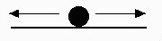
Fig. 4.2a. Neutral stability. Analogy: Marble on a flat surface (plane).
Marble will tend to stay wherever it is moved to.Local stability — this occurs when a small perturbation of the system
will tend to return to the starting point. The local stability may not, however, extend globally.
Intermediate level of stability.
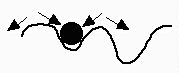
Fig. 4.2b. Local stability. Analogy: Marble in a local trough. Marble will return to starting point for small shifts, but larger shifts will lead to attraction to a new equilibrium state (a different trough).
Global stability — this occurs when even a large perturbation returns to the starting point. Start anywhere
and the system will return to the same starting point.
The strongest form of stability.
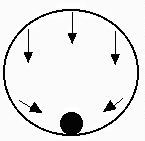
Fig. 4.2c. Global stability. Analogy: Marble in an enclosed sphere.
Marble will return to the bottom of the sphere from any position.
Food for thought: how would you draw a marble cartoon for an unstable equilibrium ?
When is
exponential
growth stable? Mathematically, this means that the rate of change is
zero
-- the system is at equilibrium. Verbally, it means the
population
will neither grow nor shrink. The equation we started with
dN/dt = rN
is a rate of change equation
(it describes the slope of the plot of population size against time).
When does the change = 0?
The left-hand side describes change over time. That means that
there
is no change when the right-hand-side = 0.
(I may use RHS and LHS as abbreviations for right and left hand
side
of equations)
1) A not-very-interesting case where the RHS = 0 is when N = 0. Obviously, if we have no animals, the population won't tend to increase or decrease.
2) The other (slightly more interesting) case is when r = 0. In that case, the population will tend to stay where it is. This is neutral stability -- if the population size changes (say through a factor we are currently ignoring such as immigration) there will not be a tendency to return to the starting point. Here the conditions for stability are almost trivial. With more complicated and realistic equations, stability analysis can become more technically challenging, but the basic logic is the same.
[Think about stability conditions for the equation for logistic growth in Lecture 5, for example].
Now let's go back and actually solve the differential equation
dN/dt = rN (Eqn 4.6)
so that we have an explicit
solution
for N(t) [the population size, N, at time t;
can also be written as Nt ].
We begin by
"separating
the variables" (N's on one side with dN, r on the other with dt) to give
(Eqn 4.7)
Next, we integrate both sides of the above. The left hand side (LHS) with respect to N, the right hand side (RHS) with respect to t, using the definite integral for the N, from the starting size Nø to the current size Nt .
(Eqn 4.8)
Now, the integral of 1/x
is
the
natural logarithm of x, ln[x], and definite integrals
are
solved by subtracting the
"starting solution" (ln[Nø])
from the "ending solution" (ln[N t]).
Remember from basic calculus that the integral of a constant (we are assuming that r is constant) with respect to x is simply x times the constant, so the integral of r with respect to t (i.e., the right hand side of Eqn 4.8) is simply rt. Given those modifications we can rewrite Eqn 4.8 as:
ln[Nt ]- ln[Nø] = rt (Eqn 4.9)
If we simply want to calculate r from empirical data (as in Homework 1) we can use
(Eqn 4.9a)
But the difference between the logs of two numbers = the log of their quotient -- e.g., ln[10] - ln[2] = ln[5] -- , so we can write:
(Eqn 4.10)
Now exponentiate both sides (raise e to the power of the terms on each side; remember that, for example, eln(2) = 2) to get
(Eqn 4.11)
Move the Nø to the right hand side and we've solved for Nt in terms of our starting population, Nø, and the growth rate, r:
{Q.E.D. is Quod Erat Demonstrandum, meaning "which was to be shown" in Latin}
Units: what are the units of r? Use Equation 4.9a, and the fact that the difference between logs is the same as the log of the ratios, to figure out the units of r.
A quantity that is sometimes of interest is the doubling time — the time it takes a population to double in size under positive exponential growth. This is well covered in the Gotelli text (pp. 6-9).
We can calculate the doubling time from any one point to any other (it is constant) so it is convenient to start with Nø, our starting population size (because, as we will see, that allows us to cancel the Nø terms completely). The trick here is to make our population at time t (Nt) be twice the starting population.
2Nø = Nø ert (Eqn 4.13)
[All we did was replace the N t of Eqn 4.12 with 2Nø]. Right away we can cancel the Nø, then take the log of both sides, giving us ln(2) = rt or
The faster the population growth, the shorter the doubling time.
(Eqn 4.14)
If the population is growing exponentially (as we have assumed here) the doubling time is a constant -- that is, if r is, let's say 0.1, then the doubling time is 6.932 regardless of whether the current population size is 100 or 1,000,000.
Let's examine the growth rate, little r and compare it to a related measure, l (lambda), which we will be using extensively when we deal with matrix-based models.
r is sometimes called the
intrinsic
or instantaneous rate of increase or "little r." It
expresses
the balance between inflow and outflow
(e.g., r = b - d
after the first equal sign in Eqn. 4.5 ).
l is called the finite rate of increase. It is the factor by
which the population is multiplied per time unit.
You should definitely memorize the following relationships:r = ln[l] (Eqn 4.16)
The table above tells us that a population is:Declining Stationary Growing
r - infinity to <0 0 > 0 to + infinity (range from - infinity to + infinity)
l 0 to <1 1 > 1 to + infinity (range from 0 to + infinity)
l cannot be negative (it's something we use to multiply the animals by, and we
can't have negative animals),
but
r can be negative
(we can have a negative interest rate, or put differently, er
is a fraction, not a negative number).
** See the WyoWeb reading from the Krebs ecology text for a discussion of finite (l) and instantaneous (r) rates. **
[A useful approximation: when r is very near zero (and therefore l
is very near 1.0) we can also use
the approximation that l
is approximately equal to r + 1].
§§§§§§§§§§§§§§§ §§§§§§§§§§§§§§§ §§§§§§§§§§§§§§§§§ §§§§§§§§§§§§§§§§§§ §§§§§§§§§§§§§§§ §§§§§§§§§§References:
Hardy, G.H.. 1992 (1st. edn. 1940). A Mathematician's Apology. Cambridge Univ. Press. Cambridge. [Apology here does not mean "I'm sorry", rather it means "here's what makes me tick". This is the Hardy of Hardy-Weinberg that we will cover later in the semester]Krebs, C.J. 1994. Ecology (4th edn.). Addison Wesley Longman, NY.
Maynard Smith. 1982. Evolution and the Theory of Games. Cambridge Univ. Press, Cambridge.
Wilson, E.O., and W.H. Bossert. 1971. A Primer of Population Biology, Sinauer Associates, Sunderland MA.
URL: http://www.sinauer.com/
Return to top of page Go forward to notes for Lecture 5, 25-Jan