How did we get these Cavalli-Sforza distances? They are simply a geometric view of the distances between multi-dimensional points on a hypersphere (a sphere with > 3 dimensions). Say we have two subpopulations S1 and S2 assayed at a single locus with alleles i = 1 to k. The formal definition is:
 Eqn 6.1
That is, we take the square root of the frequency of allele 1 in S1 times that of allele 1 in S2 and repeat and sum that quantity for all k alleles. That gives us Cos (y) which we can plug into the square-root term on the RHS (right hand side) of Eqn 5.1 above. I don�t expect you to use or memorize this -- just to see that it is a purely numerical/geometric approach. If we were doing it in 3 dimensions it would be akin to figuring out the distance from New York to London along the surface of the globe (called the chord distance). It can be fairly easily incorporated into a number-crunching computer program that will produce output like the table of Cavalli-Sforza distances shown above. Those distances, in matrix form, can then be used as input for phylogenetic tree-building routines such as the UPGMA, Fitch-Margoliash and neighbor-joining approaches we used in the homeworks.
The Cavalli-Sforza chord distance was an early measure and is still used (in fact I see it gaining ground for use with microsatellites). Another geometric distance that was widely used with allozymes (but I have not seen used with microsatellite data) is Rogers� distance (Wright, 1978). One reason the Cavalli-Sforza distance may be in greater current use is that it was specifically evaluated (and performed well) in simulations of tree-building algorithms by Takezaki and Nei (1996). [For all we know Roger�s distance may perform equally well or better under circumstances that would apply well to the questions people like me seek to address -- but since no one has done such a study, people like me will tend to go with one that has a documented good track record]. A very important part of the robustness of a distance measure is its performance under a variety of conditions. It is always best if we can compare several distance measures under conditions in which we know what the answer should be. Paetkau et al. (1997) provide an evaluation of various distance measures that apply to distance measures potentially useful for microsatellite analysis of bear populations.
2) Distance methods with biological assumptions. With a little luck (or a lot of hard work), we know something about the evolutionary forces (most importantly here mutation and drift, since we assume we are using markers that are not subject to natural selection) driving genetic change in the system we're interested in. If so, it seems reasonable to take advantage of that knowledge by incorporating it into building a distance model. After all, we expect models with greater realism to perform better (albeit at the cost of greater complexity, usually). Several distance measures incorporate assumptions about the importance of drift and mutation as forces of change:
Reynolds� distance or the "coancestry" distance (Reynolds
et al., 1983; see Weir, 1996, p. 167)
Nei�s distance (Nei 1972, 1978)
Models using a stepwise mutation model (SMM) specifically
developed for microsatellites (e.g., dm2[delta
mu squared] of Goldstein et al., 1995).
The problem with making assumptions is that violations
can cause errors. Empirically, it appears that many of the stepwise mutation
models for microsatellites do not perform well when analyzing many (most?)
data sets, especially those where small population sizes mean that drift
has played at least as large a role as mutation. Reynolds� distance, which
was derived for allozyme data on small (e.g., vertebrate) populations assumes
a primary role for drift and is an infinite-alleles model (an allele can
change from any given state into any other given state). Reynolds� reliance
on "drift only" seemed inappropriate for microsatellites, which
have:
a) a mutation rate that appeared clearly much larger than that
of allozymes (1 mutation per 1,000 or 10,000 replication events for microsatellites
vs. 1 mutation per 1,000,000 replication events for allozymes). [But that
may be based on very long repeats in highly polymorphic human populations].
b) a mutation process that would seemingly not fit the infinite-alleles
model because mutations generally occur in "stepwise" fashion by adding
or deleting one of a series of beads (AC10 goes to AC9 or AC11, where the
subscript refers to the number of AC repeat units).
[See my web page http://www.uwyo.edu/zoology/mcdonald/dna.htm for a
quick overview of microsatellites].
Nevertheless, Reynolds' distance and its neglect of the importance
of mutation, may work better than we would have expected (at least
in some species/populations) for two reasons:
a) small population sizes (= high potential for drift)
b) "missing steps" because drift creates a "chunky" distribution of
alleles instead of the smooth bell curve we would expect under a strict
stepwise process.

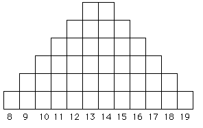
Fig. 6.1. A microsatellite allele frequency
distribution under a strict stepwise mutation model (SMM). The X-axis
shows the number of repeat units (e.g., AC8 to AC19),
while the Y-axis shows the number of alleles. Starting with either
a 13 or 14 repeat chain as the ancestor, we tend to accumulate more
alleles at sizes close to the starting point because of equal likelihood
of additions or subtractions and because larger changes (a variant of "mutations of large effect") will tend to be rare (we think).

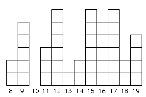
Fig. 6.2. An allele frequency distribution that has been greatly affected by drift and may better fit an infinite-alleles model (IAM). Even if the mutations that generated the original variation did occur in stepwise fashion, drift has removed some allele sizes (e.g., the 10-repeat category) while randomly selecting others to be greatly over-represented (e.g., 12, 15 and 17). This sort of "chunky" distribution may be quite common in many natural populations of vertebrates (where effective population sizes, Ne, are always small or at least often fluctuate to low numbers).