Converting an lxmx schedule into a Leslie matrix.
Should we convert an lxmx schedule? When will the answer be yes, and when will it be no?YES: If we are interested in analyzing some published data that already exist in lxmx format (perhaps to compare with data we have collected or for comparison with another data set of our own or from the literature)
NO: if we were starting a field study from scratch and plan to use them in a matrix format (then we would calculate the Pi and mi directly from our data)
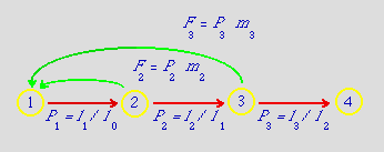
First, let's look at the life cycle graph:

Fig. 12.1.
Life
cycle graph for a birth-pulse age-classified population with a
post-breeding
census.
The terms are designed to show the data used for
calculating the parameters from the lxmx
table below.
Let's look at a completely age-classified life cycle for which someone has tabulated an lxmx data set. The lxmx format is a traditional one from which one can calculate many of the same "outputs" such as reproductive values and the stable age distribution. The matrix format though, allows us to do everything we can do with the lxmx table and considerably more. Here's an example of an lxmx table:
Table 12.1. lxmx schedule used to formulate a life cycle graph like that of Fig. 12.4.
2 0.315 1
3 0.2205 3
4
0
0
________________________________
[Note that lxmx tables will sometimes have an implicit zero for the last line. I show zeros just to emphasize that we will often use an all-zero column in our matrix]
From continuous x to discrete i: Note that we are moving from continuous age (x) to discrete age class (i). Refer back to Fig. 12.2 to remind yourself of the distinction between continuous age (subscripted x) and discrete age-class (subscripted i).
Fertilities: Conveniently, though, the mx = mi. Try the logic. First-year individuals (i= 1) reproduce at the end of their first year when they are 1 year old (x = 1). Similarly mi = mx for all older age classes.Let's use the equivalences we just developed to turn the lxmx data in Table 12.1 into the Pi and Fi that we use in the Leslie matrix.Survival rates: For a post-breeding census Pi = lx=i / lx-1.
With those two equivalences we can turn any lxmx schedule into the corresponding Pi and Fi terms needed for the life cycle graph and matrix in a matrix-based analysis.
P2 = l2 / l1 = 0.315/.45 = 0.70
P3 = l3 / l2 = .2205/0.315 = 0.70
P4 = l4 / l3 = 0/0.2205 = 0
F1 = P1 * m1 = 0.45 * 0 = 0
F2 = P2 * m2 = 0.70 *1 = 0.70
F3 = P3 * m3 = 0.7 * 3 = 2.1
F4 = P4 * m4 = 0 * 0 = 0
| F1 | F2 | F3 | F4 |
| P1 | |||
| P2 | |||
| P3 |
Top row (fertilities) and subdiagonal (survival): Note that, for a strictly age-classified analysis, fertilities will be in the top row and annual survival rates in the subdiagonal. All the other cells are empty (zero). As we will see in the Sage Grouse example, however, stage-classified life cycles can have non-zero cells in other places (they will almost always still have the fertilities in the top row, though).
Plugging in the values from above we get
the following
numeric values:
| 0 | 0.70 | 2.10 | 0 |
| 0.45 | |||
| 0.70 | |||
| 0.70 |
Now we can crunch the matrix with a matrix demographic analysis package.
§§§§§§§§§§§§§§§§§§§§§§§§§§§§§§§§§§§§§§§§§§§§§§§§§§§§§§§§§§§§§§§