Lecture notes for ZOO 4400/5400 Population Ecology
Return to Main Index page
Go back to notes for Lecture 11, 8-Feb
Go forward to notes for Lecture 13, 13-Feb
Go to notes
on matrix algebra (e.g., how to multiply matrices)
Go to glossary of matrix algebra terms
Download Excel spreadsheet for projecting a census vector
Go to notes on converting an lxmx
table into a matrix
Download Excel spreadsheet for working with lxmx schedule
This spreadsheet also illustrates how to calculate sensitivities from the reproductive value vector (RV, left eigenvector) and the stable (st)age distribution (SSD, right eigenvector).
Approach III: The life cycle graph [The best place to start formulating a model]
The problem with the two formulations in Eqns 11.1 and Eqn 11.2 (equations and matrix) is
that they are difficult to visualize in terms of the natural history of the organism of interest. Eqn 11.2
is great for computers, but not easy to think about when trying to put the life history of the organism one is interested in into a matrix
model setup.
The best way to play with possible ways to set up a matrix-based analysis
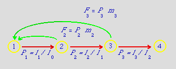
is by the use of a life cycle graph, such as the one shown below.

Fig. 12.1.
A life
cycle graph corresponding to Eqns 11.1 and the matrix
formulation
of Eqn 11.2 and Fig. 11.1
(redone as a figure in Fig
12.3).
The four nodes (yellow circles)
depict four age classes.
The red arcs (arrows) depict transition
probabilities between age classes (in the case of a strictly age-classified
matrix, these will be age-specific survival rates).
The green arcs depict fertilities, the production of new recruits. Note that the green arcs (Fi)
are compound terms including the survival of the parents (Pi), as well as offspring
production
(mi).
This is a result of a post-breeding census approach that I will explain below.
Although we
are using single subscripts here (Fi, Pi)
the more general way to refer to the arcs is as the aij
(arc from Node j to Node i).
Thus F3
is equivalent to a13. The P1 = l1/l0 is to show how one
converts the entries in an lx table into the matrix survival entries.
How and when births occur makes a big difference:
All of the above (Eqns 11.1, Eqn 11.2, Fig.
11.1 and Fig. 12.1) represent analysis of a discrete birth pulse (once a year pulse of breeding)
post-breeding census formulation. That is, immediately after the annual birth pulse
(spring or summer for many birds and mammals in North America), we census the population. It will consist of newborns (first-year individuals),
second-year individuals (that have just celebrated their first birthdays),
third-year individuals (just celebrated their second birthdays) and fourth-year
individuals. The fourth-year will not survive to the next birth pulse (hence the
lack of an arc from the fourth node back to the first). Compare the matrix of Eqn 11.2 or Fig. 12.3 care fully with
the life cycle graph of Fig. 12.1.

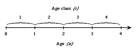
Fig. 12.2.
Difference between discrete age class
(subscripted i) used in matrix projection models and continuous age (x) used, for
example in lxmx life table analyses.
Age classes are discrete (time goes in steps or "chunks" as opposed to
flowing continuously). That is, age classes are first, second,
third, etc. Individuals are "first-year" from the time
they are born (and censused) until just before their first birthday. From Caswell, (2000), which is the best single source for learning matrix model
approaches. Jenkins (1988) focused especially
on the problems of indexing that have confused even very good ecologists.
Gotelli’s 1st edition had an error in computing reproductive
values that was due to an indexing problem (Steve Jenkins is acknowledged in the Preface to the 2nd edition for finding the error).
The formulations above all represent an annual census taken just after the birth pulse. Strictly speaking, we make the assumption
that all members of the population reproduce on the same day and that all the newborns and birthday celebrants are then immediately censused (in
practice one would try to have the census at the end of a breeding season that is presumably short compared to the census interval (i.e.,
census takes a few days within a 1-yr census interval). We can use census intervals other than years but all census intervals must be equal
(we can't assess some transitions that occur with a 6-month interval and others that are annual).
If we conduct a pre-breeding census then instead of following the survival of the parents along the reproductive arcs, we
must follow the survival of the newborns from birth until we actually
census
them almost a year later. The life cycle graph's terms then look like
the
formulation below. [For most vertebrate populations it makes more sense
to do a post-breeding census]. See Caswell
(2000) for more
details on formulating a pre-breeding matrix model. [Personally,
I almost always work with a post-breeding census].
Here's a symbolic matrix corresponding to the life cycle graph of Fig. 12.1.
Fig. 12.3. Projection matrix
corresponding to the life cycle graph (LCG) of Fig. 12.1. The
top row elements are the fertilities (Fi
= Pi * mi) and the subdiagonal elements are survival rates (
Pi).
Note that, for a strictly age-classified analysis, fertilities
will be in the top row and annual survival rates in the subdiagonal.
All the other cells are empty (zero). As we will see in the Greater Sage-Grouse
example, however, stage-classified life cycles can have non-zero
cells in other places (they will almost always still have the fertilities in the top row, though).
Here are some specific numerical values for the vital rates:
m2 = 1 (1 female offspring per second-year female
breeder)
m3 = 3 (3 female offspring per second-year
female breeder)
P1 = 0.45 (45% annual survival from birth census to
end of first year)
P2 = 0.7 (70% annual survival through second year)
P3 = 0.7 (70% annual survival through third year)
No animals survive to breed at the end of their fourth year
Plugging in the values from above we get the following numeric values:
| 0 |
0.70 |
2.10 |
0 |
| 0.45 |
|
|
|
| |
0.70 |
|
|
| |
|
0.70 |
|
Now we crunch that with a matrix demographic analysis package and come up with:
l = 0.99 (the population is almost stationary; stationary means it is neither
growing nor shrinking; we use this term to avoid confusion with the term "stable", which has a special meaning referring to the equilibrium
reached when the transient dynamics yield to a population that grows with a
constant proportion of individuals in each age-class or stage -- the stable
(st)age distribution). At that equilibrium the "stable" population may
still be growing very rapidly or it may be declining rapidly. What isn't changing is the
proportion of individuals in each of the age-classes or stages.
Stable age distribution: (because it is a right eigenvector, this one is a vertical 4X1 vector)
0.499
0.227
0.160
0.113
Reproductive values: (a left eigenvector will be a horizontal 1X4 vector) {1., 2.20, 2.12, 0}
Note that the reproductive value of the fourth-year individuals is 0.
That's because they will not survive to reproduce again.
Typically reproductive value curves peak at the age of first reproduction because
they measure current reproduction plus all future reproduction discounted by the probability
of surviving to reproduce in the future. Note also that reproductive values and stable age distribution
are properties of an age-class or stage (the nodes), while sensitivities and elasticities are
properties of a transition (the arcs).
Scalar product (SP): 1.3389. {Not
required: We can calculate the scalar product as the sum of the cross-products
of the corresponding elements of the two eigenvectors. That is, 1 * 0.499 + 2. 2 * 0.227 + 2.12 * 0.16 + 0 * 0.113 = 1.3389}.
Suggestion for building on skills worked on in Homework 3: use the formula
sij
= (RVi*SADj)
/ SP
[Eqn 12.1]
to be sure you can calculate sensitivities correctly. RV is the reproductive value vector, SSD is the stable stage distribution vector.
{Remember, aij is the transition from Node j to Node i. Also, arc is
the element in the rth row and cth column
of the matrix. I like to use the correspondence P1
= a21 = survival from first-year to second-year to remind me how keep the subscripts straight.
For example, s43 would be the sensitivity of lambda to a change in the
vital rate that goes from Node 3 to Node 4}.
Sensitivities shown below: (only the "possible"
values are listed). The sensitivities tell us the effect on l of an additive change in a vital rate.
| 0 |
0.169 |
0.12 |
0 |
| 0.822
|
|
|
|
| |
0.359 |
|
|
| |
|
0 |
|
Small changes in first-year survival would have the biggest impact on l, followed by second-year
survival and then second-year reproduction.
As shown by Eqn 12.1, the sensitivities are cross-products of a right
eigenvector element (which has as many elements as the graph has
nodes/stages) and a left eigenvector element. Qualitatively, the
sensitivity of l to each arc is the product of the SSD (Stable Stage
Distribution = how many) of the source node, times the RV (reproductive value = how valuable) of the target node.
Sensitivity of arc to Node i from Node j = SSD of Node j times RV of Node i.
= “how many” in the source times “
how valuable” is the target?
If we have lots of individuals in the age-class (node) that the arrow is coming from (big SSD value), and the arrow is pointing to a
very valuable node (high RV), then changing that arrow (aij) will have a big impact on l.
The whole point of eigenanalysis is to tell us how a matrix (of vital rates) affects a
vector (a count of the animals in the age-classes or stages) – the matrix is a multi-dimensional object that transforms
what it multiplies. For us, the matrix is a demographic projection
matrix (set of vital rates) and the vector it is affecting is a census
vector (the population count, categorized by age or stage). The
dominant eigenvalue (l) tells us how fast the projection matrix grows or
shrinks the population – the growth rate. The two eigenvectors
tell us two different but important things about how the projection
matrix acts. The left eigenvector (reproductive values, RV) tells us
which ages or stages have the biggest per capita role in producing that
growing or shrinking – sort of the power of that stage (do we have
pawns, knights or queens in our forces?). The right eigenvector
(the stable stage distribution, SSD) tells us how many of each of the age
classes or stages we will have (how many pawns, knights or queens are
in our army?). Multiplying importance (left eigenvector elements)
by how many (right eigenvector elements) tells us how much of an effect
that arc (vital rate, or transition between stages) will have on
l. If our chess move (the arc or vital rate) involves a large
cohort of queens, it will have much more effect than if it involves a
small force of pawns. It will take many pawns to have the same
effect as one queen. One or two knights may not be a match for a
large force of pawns. We can trade off number (SSD of source)
against importance (RV of target) in determining sensitivity.
Elasticities:
The elasticities are calculated from the formula:
eij = (sij * aij)/l
[Eqn 12.2]
That is, they are the sensitivities (sij) times the original matrix entries (aij, arc values)
all divided by lambda. (See also the table at the bottom of the notes for Lecture 11). The elasticities will always sum to 1.0. Putting the elasticities into a matrix we get:
| 0 |
0.120 |
0.254 |
0 |
| 0.373 |
|
|
|
| |
0.254 |
|
|
| |
|
0 |
|
Notice that the second-year survival and third-year reproduction are now much more nearly equal in importance to first-year survival.
The elasticities tell us the effect on l of a proportional
change in a vital rate.
m1 (cohort generation time) = 2.68 (years). The pace of evolution is largely determined
by generation time (remember back to my contrast between the growth rates of Iceland and Ireland in Lecture 8 -- that difference
is largely due to the shorter generation time in Iceland). Bacteria can evolve much more quickly than can elephants
or humans because of their much shorter generation time. m1 is the mean of the discrete equivalent of the
lxmx schedule (or net maternity function). The skewness and kurtosis of the
lxmx distribution are also of interest. The skewness is the third moment
of the distribution (first is the mean, second is the variance), while the kurtosis is the fourth moment. Skewness tells us how drawn-out the tails of a distribution are, kurtosis tells us how peaked (leptokurtic) or flat (platykurtic)
a curve is. Together these moments determine the shape of the curve, and can tell us a great deal about the life history of
the organism. For example, if reproduction is spread out over the lifespan, the curve
(plot of lxmx against age) will be flat (platykurtic).
Hint: Make sure to distinguish between arc-related measures and node-related
measures.
Look at several examples of life cycle graphs (or matrices). Each
has a certain number of stages or age-classes (equal to the number of
rows and to the number of columns in the projection matrix). The
eigenvectors have exactly that many elements – they relate directly to
nodes/stages rather than to arcs. Each of the elements of either
the SSD or the RV vectors has a one-to-one correspondence to one of the
stages. Now look at the arcs (transitions, vital rates) in a
variety of life cycle graphs. The graph will have at least as
many arcs as it has nodes/stages. The number of arcs is the same
as the number of non-zero elements in the projection matrix. Any
particular node may have several incoming and several outgoing
arcs. Most matrices will have many more non-zero cells than they
do rows or columns. The sensitivities and elasticities relate to
arcs/transitions rather than to nodes. Put differently, they
involve the relationship (connecting arrow) between two different
stages (or back to the same stage in the case of self-loops). In
fact, we can compute sensitivities for transitions that don't even
occur on the life cycle graph. That is, we can ask a sort of
“what if” question for the importance of non-existent transitions (this
is why I often restrict my attention to the “possible” sensitivities –
those that correspond to non-zero cells or existing arcs in the life
cycle graph. Often the non-existent arcs are meaningless
(transition from age four to age two is unlikely to yield much
insight), but occasionally a non-existent arc is plausible, even if not
yet observed (e.g. reproduction at earlier stages by organisms with
delayed reproduction).
References:
Caswell,
H. 2000. Matrix Population Models (2nd Edn.). Sinauer Associates, Sunderland, MA
McDonald,
D.B., and H. Caswell. 1993. Matrix models for avian demography. Chapter
10 In Current Ornithology Vol. 10 (D. Powers, ed.). Plenum Publishing, NY
Cochran,
M.E., and Ellner, S. 1992. Simple methods for calculating age-based life
history parameters for stage-structured populations, Ecol. Monogr. 62: 345-364.
van Groenendael, J., H. de Kroon, S. Kalisz, and S. Tuljapurkar. 1994. Loop analysis:
evaluating life history pathways in population projection matrices. Ecol. 75: 2410-2415.
Wisdom, M.J., and L.S. Mills, 1997. Sensitivity analysis to guide population
recovery: prairie-chickens as an example. J. Wildlife Mgmnt 61: 302-312.
§§§§§§§§§§§§§§§§§§§§§§§§§§§§§§§§§§§§§§§§§§§§§§§§§§§§§§§§§§§§§§§
Return to top of page
Go
forward to notes for Lecture 13, 13-Feb

