Lecture 32 (19-Apr-13)
Return to Main Index page Go back to notes for Lecture 31, 17-Apr Go forward to Lecture 33 21-Apr-13
The spread of infectious diseases (continued).
Last time, I introduced a simple difference (discrete) equation model for the spread of an infectious disease.
which has the following equilibrium value (I*)Eqn 32.1 (= Eqn 31.2)
Eqn 32.2 (= Eqn 31.8)
What does equilibrium mean here? It means that there will be no change in the infection level -- that is the rate of addition of new infections will be balanced by the recovery rate (a population growth analog would be dN/dt = 0 when births = deaths) .
We also solved for some aspects of the graph of It as a function of time. We know its Y-intercept, given by:
Working with empirical data for the observed spread of an infectious disease.and its slope given by{Y-intercept} Eqn 32.3 (= Eqn 31.4)
m = (1 - g - r) {slope} Eqn 32.4 (= Eqn 31.5)
Let's say we have an empirically observed plot of It values over time. We have only two equations (Eqn 32.3 = Eqn 31.4 and Eqn 32.4 = 31.5) for three unknowns, L, g, and r -- too few equations to solve for the unknowns. We can, however, use some tricks, based on other knowledge about constraints on the system, to obtain estimates of these unknown parameters from the data.
First, let's find the equilibrium solution from the observed data. Remember from Eqns 32.3 and 32.4 that gL and (1 - g - r) are the intercept and slope respectively. But the equilibrium [Eqn 32.2] is just the intercept (gL) divided by 1 minus the slope [1 - (1 - g - r) = g + r], so we can calculate the equilibrium value
If we calculate the slope from ordinary least squares regression (that is, by analyzing the numerical values of the data points statistically) or simply by using a cruder rise-over-run approach on a graph, we'll then be able to calculate the equilibrium level of infection. Next let's look at reasonable bounds on g.Eqn 32.5
soEqn 32.6 (= Eqn 32.3 = Eqn 31.4)
But we know that 0 and 1.0 are the bounds on the possible values of L, so we can rewrite Eqn 32.7 as an inequalityEqn 32.7
Look just at the b/g < 1 and multiply both sides by g to get b < g which we can reverse as:Eqn 32.8
g > b Eqn 32.9
That is, g (the infection rate per unit time) will be greater than the Y-intercept of our empirical plot. We now have a lower bound for g. Let's use similar logic to calculate an upper bound. Remember from Eqn 32.4 that the slope is given by
m = (1-g-r) {slope} Eqn 32.10 (= Eqn 32.4 = Eqn 31.5)which can be rearranged to solve for r as
r = 1-g-m Eqn 32.11As for L, r lies in the interval 0 to 1.0, so
0 < 1-g-m < 1 Eqn 32.12Now just move the g to the left of the inequality (and ignore the fact that it is, of course < 1), so that we now know that
g < 1-m Eqn 32.13
That is, we now know that the upper limit for g is given by 1 minus the slope (m) of our empirical plot.
Combine Eqns 32.9 and 32.13 together for the upper and lower bounds on g
b < g < 1-m Eqn 32.14Let's make the reasonable assumption that the possible estimates of g are normally distributed (i.e., the values fit a bell-shaped curve) over the interval from b to 1 - m. The maximum likelihood estimator of g is then the midpoint of that interval. [§§ We could use a more complex maximum likelihood estimator (MLE) for other kinds of distributions §§]. This gives us an estimate of g as
where the "hat" over the variable denotes the fact that it is an estimate. That "solved" for one of the three (too many) unknowns. Now we can solve for the other two (just enough) unknowns. SubstitutingEqn 32.15
and substitutingEqn 32.16
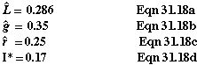
Let's say that our observed data had an intercept, b, of 0.1 and slope, m, of 0.4. We then obtain estimates ofEqn 32.17
[Note: all the above should be Eqn 32.18 not 31.18] We have used knowledge of constraints on the system to calculate equilibrium values and parameter estimates from relatively little information. From the observed infection data we have been able to estimate
1) the rate of spread (g),
2) the rate of recovery (r), and
3) the upper level of proportion infectable (L).
Having an estimate of any one of those three previously unknown parameters could be very useful in managing a population subject to infectious disease. Estimating them directly would be very difficult. Doing the empirical plot of It+1 against It is much more feasible, and is all we really need.
References:
Huckfeldt,
R.R., C.W. Kohfeld, and T.W. Likens. 1993. Dynamic Modeling: An Introduction.
Quant. Applic. Soc. Sciences No. 27.
Sage University Press, Thousand Oaks, CA
§§§§ §§§§§§§§§§§ §§§§§§§§§§§§§ §§§§§§§§§§§§§§§§§§§§§§§§§§§ §§§§§§§§