Lecture
notes for ZOO 4400/5400 Population Ecology
Lecture
11,
(Friday, 8-Feb-13)
Matrix population
models.
Return
to Main Index page Go
back to notes for Lecture 10, 6-Feb Go
forward to notes for Lecture 12, 11-Feb
Go
to glossary
of matrix algebra terms
Required reading: Gotelli text, pp. 56-79
Suggested reading:
McDonald, A primer for stage-classified life cycle graphs (on WyoWeb)
Suggested reading: McDonald, Demographic
analyses of mating systems (on WyoWeb)
Suggested reading: van Groenedael, Projection
matrices in population biology (on WyoWeb)
Matrix-based
approaches to the analysis
of single populations.
For the first few lectures I talked about
exponential
and logistic models for the growth of single populations. Obviously though, populations
can't grow or decline
(at least in the long term) without filling the universe or going
extinct.
Most populations therefore have r = 0 or l=1.
We will now study a useful method for analyzing single-population
dynamics
-- matrix-based approaches -- many of whose most powerful insights will
have little to do with whether the population is increasing or
decreasing.
I will give a brief general introduction and then work through an
actual
case history. Once we've seen a little bit about how and why this
kind of approach might be useful, we'll delve into more detail on the
techniques
used.
Outside readings: van
Groenendael
et al. (1988) is a good reading for an overview of what the
approach
can do. It will be a "suggested" but not required reading, and
I have put a copy in the WyoWeb folder. Caswell
( 2001) has written a
book on the subject that is the single comprehensive source for this
major
approach to modeling population dynamics. I wrote a book chapter
with Hal Caswell that some of you may find useful (McDonald
and Caswell, 1993), and I have also put in the WyoWeb folder a
"primer"
I wrote on matrix models.
One of the things we ignored in the
exponential and
logistic models was the role of age structure. For almost any organism
it's reasonably obvious that age (or size) makes a big difference to
the
role of an individual in a population -- as we saw in looking at some
of
the broad patterns of natality and survival in natural
populations.
Both the birth rates (female offspring per female) and the survival
rates
will usually change as a function of age. In some species (e.g.,
fish, trees) with indeterminate growth, size will be a major
determinant
of birth and survival rates --- large individuals will produce more
offspring
and have higher survival rates. Matrix models are flexible enough
to allow us to classify individuals by size as well as age -- this may
be very useful, for example, when analyzing the dynamics of fish or
insect
populations, where size rather than age is the major determinant of
reproductive
output and sometimes survival.
So let's see about developing the
matrix-based approach
that allows us to do that.
Matrix projection models--an
under-utilized demographic
tool.
1. Historical origins--the Leslie matrix (Leslie,
1945)
Fig. 11.1. An (age-classified) Leslie matrix with fertilities in the
top row and
survival rates along the subdiagonal. The fertility and survival
rates are collectively called the vital rates.
We can use this matrix to project population growth from a census
vector
(a count of the individuals in each age-class). This matrix has 3
age-classes (the matrix is 3-by-3).
Compare and contrast this matrix with the equations and matrix of Eqn
11.2 and Fig. 11.1 and the
corresponding
life cycle graph shown in Fig. 11.2.
2. Setting up the model (Caswell
2001; McDonald & Caswell, 1993)
a) Why are we doing a demographic analysis?
What won't we get?
b) Deciding what kinds of transitions matter
c) The problem of missing or incomplete data
d) Parameterization -- putting in the survival and
reproduction terms (vital rates). More on this later
e) A guide to future field work. Matrix models tell
us about the transitions in the life cycle to which the population growth rate (l) is sensitive or elastic -- these terms mean that changes in those vital rates will have a big impact
on the population growth rate. If a transition is highly sensitive,
then we need very accurate measurements of any component terms such as
survival rates, because inaccurate values will yield an inaccurate
analysis. On the other hand, insensitive arcs suggest places where one should not
overdo the effort (many ornithologists spend too much time and effort assessing
nesting success and not enough assessing survival).
N.B. Even if a transition
is highly sensitive it doesn't mean we can do anything about it. A manager may have to weigh the cost and feasibility of acting on the
most sensitive transitions against the practical reality that it may be easier
to do something about a relatively insensitive transition.
3. The major outputs:
Lambda (l) the population growth rate (at equilibrium).
Usually close to 1.0 (1.0 = stationary,
neither growing nor shrinking).
Sensitivity--what effect does an absolute change in a vital rate (arc in the life cycle graph or cell in the
matrix) have on l?
For example, if we change first-year survival by 0.01, how much will that affect the
population growth rate?
Elasticity--what effect does a proportional change in an arc (vital rate) have on l?
For example, if we change first-year survival by 1%, how much will that affect population growth?
Stable (st)age distribution--proportion of the population
in each (st)age.
What proportion of the total population are first-year individuals?
Second-year individuals? Etc.
At equilibrium, a population's age structure won't change, even if the population is growing or shrinking.
Reproductive value -- value of a given age-class or stage as a seed for population growth
(newborn or first age class reproductive value = 1.0 by definition).
Example: an adult female sea turtle is "worth" 588 turtle eggs
(Crowder 1994).
4. Comparing life histories (quantitatively!)
a) Using the elasticity vs. the sensitivity. Elasticity assesses effect of a proportional change in the values,
whereas the
sensitivities assess the effect of an additive change.
b) Matrix output gives us a whole suite of parameters to compare among populations and species.
Some other tools and data requirements:
i. We will usually want robust estimates of
survival rates from mark-recapture (e.g., mist netting) data
ii. Basic natural history: if you don't know your organism well, you may overlook critical life history transitions.
iii. Incorporating greater realism by accounting for demographic stochasticity (important in small populations) vs.
environmental
stochasticity (can be important even to large populations)
iv. Another important addition is to incorporate density dependence: how does density affect birth rates, mortality and other
vital rates? Our initial matrix models will ignore density dependence. That is, the vital rates will be constant through time and over all population sizes.
Real-world examples:
Matrix models of sensitive species in Forest Service Region 2 (including WY). Assessment of population of black-footed ferrets in Badlands National Park and adjacent Buffalo Gap National Grassland
in South Dakota. Population has grown to over 200 free-living ferrets from the captive-bred founders.
Individuals born in the wild do much better as founders for new introduced populations. Can the managers of the SD
population afford to "give away" some of their ferrets to help establish other populations? Matrix models
provide a quantitative basis to help guide management decisions. Recently, the population in the Shirley Basin, WY has shown exponential growth highlighted in a short paper in the journal Science (Grenier et al., 2007).
 Black-footed ferrets have thrived in the large black-tailed prairie dog colonies in the Conata Basin, SD. Matrix population models have helped guide their management.
A matrix population model is a demographic technique for understanding phenomena at the population
level based on information from the individual level (birth, death, and growth rates of individuals; we'll call these demographic rates the
vital rates). The major mathematical links are from equations on the one hand, and graph theory on the other hand, to the matrix
formulations that are the way computer programs actually analyze the models.
Consider a very simple life cycle with four age classes (Eqn 11.1, Fig. 11.1). We could look at population change over time in three
equivalent ways: using difference equations, using a population projection matrix (Eqn 11.2; remember the Leslie matrix from ecology
courses?) or with a life cycle graph (Fig. 12.1, in the next lecture). The three are mathematically equivalent–but their utility is context-dependent.
Approach I. Equation-based: we could use continuous differential equations (such as those we used for the exponential and
logistic) but usually use discrete, difference equations (time comes in
chunks or "intervals" as fine as days or as coarse as years). The
reason for using the discrete (vs. continuous) formulation is that many of the organisms we are interested in are pulse breeders.
That is, they have a single, relatively well-defined period (pulse) of breeding per interval
(often an annual cycle). Complex analyses of difference equations are very challenging mathematically. Complex analyses of discrete
formulations using matrix algebra are much easier (especially since the advent of the personal computer, which can handle most matrix algebra
routines with ease).
A difference equation formulation would look like this:
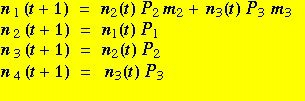 (Eqns 11.1)
The terms in the equations are ni(t), the number of individuals of age-class i at time t; Pi, the annual survival rate of individuals in age-class i, and mi, the fertilities of individuals in age-class i. The first line tells us that the number of individuals in the first age-class (n1) at time t+1 is
equal to the number of individuals (mothers) in the second age-class (n2) times their annual survival (P2)
times the number of babies they produce (m2), plus the same quantities for the third-year mothers (fourth-year individuals don't reproduce).
That is, the total babies produced equal the sum of the babies produced by the two reproductive age-classes. The second line tells us how many second-year individuals we will have at time t+1. That will be the number of babies at time t, given by n1(t), times their survival rate through the first year (P1). And so on for the two remaining age classes. Here we have an organism with four age
classes, first-year
individuals, second-year individuals, third-year individuals and
fourth-year
individuals. Fourth year individuals die on their fourth birthday just
after we have counted them (or at least before they survive through to
the next breeding season). Note also that individuals first reproduce
in
their second year. Those
birth
and survival rates are the vital rates we have discussed in the
past few lectures. For size-classified life cycles, the vital rates could also include growth rates
(Gi).
Approach II. Matrix-based: [The way we organize a demographic model for number-crunching analysis by a
computer]. Below is a Leslie matrix formulation of Eqns 11.1. Matrix algebra is just a way of organizing sets of equations in an
orderly way -- computers can easily do lots of things with matrices that would be a lot more awkward if we used sets of equations. In the first
equation of Eqns 11.1, the first-year individuals at time t+1 are a function of the number of second-year individuals at time t
times the fertility of those second-year individuals, plus the number of third-year individuals times their fertility.
All of that becomes condensed into a single matrix row-times-vector column calculation in Eqn 11.2.
We will discuss why there are "parental" survival terms in the fertility equation shortly. The matrix algebra
formulation of Eqns 11.1 can be written as:
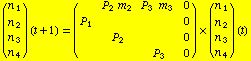 (Eqn 11.2)
In Eqn 11.2, a 4X1 census vector (LHS) at
time t+1
results from the right-multiplication of a 4X4 projection matrix by a
4X1
census vector at time t. The (mathematically equivalent
to
Eqns 11.1) matrix form shown in Eqn 11.2 is a very convenient way to
organize
Eqns. 11.1 for computer analysis. With a computer, we can do many
kinds of very powerful analyses very easily (e.g., eigenvalue and
eigenvector
analyses). The mathematical results will have biologically
meaningful
interpretations -- for example, the dominant eigenvalue of the matrix
turns
out to be the growth rate, l,
of the population. We will refer to the projection matrix (the first big
bracketed
term after the = sign in Eqn 11.2) as A (bold font, or if
writing
it by hand we can put a bar over the top), with elements aij,
referring to the element in the ith row and jth column.
(Mnemonic -- which means a way to help memorize something: R X C = Roman Catholic, rows first then columns; Arc = arc). Each
element (cell) in the matrix represents a transition (often a
probability)
of moving from the jth age class (or stage) to the ith age class (or stage). Thus, in the matrix shown above, element a21
(=P1) is the probability of surviving from the first
age class to the second. Figuring out the correct values of the
elements
(we call this parameterizing the matrix) may require hard work in
the field and always requires care in the formulation. We refer
to
these transition terms collectively as the vital rates (demographic
processes such as birth, survival, growth {in mass}, change in social
status). Given the projection matrix A, computer programs can easily calculate the
eigenvalues,
eigenvectors, and other statistics that provide insights into the
population
dynamics.
{Notation reminder: this is a projection matrix. Look back to my speedometer example for the distinction between projection and forecasting}.
Note that in Eqn
11.2 above
I have left out lots of empty cells (zeros). Another way to
write/draw
that matrix would be:
|
0
|
P2m2
|
P3m3
|
0
|
|
P1
|
0
|
0
|
0
|
|
0
|
P2
|
0
|
0
|
|
0
|
0
|
P3
|
0
|
Fig. 11.2. Leslie projection matrix corresponding to the
demographic
equations of Eqns 11.1 and to the matrix
portion
on the RHS of the matrix algebra formulation in Eqn
11.2. If we right multiply this matrix by a 4X1 census vector
at time t, the result will be the projection of the population
to
time t+1.
The only non-zero cells are in the top row
--these are
the fertilities, and in the subdiagonal (the cells below the top-left to bottom right diagonal) -- these are the annual
survival
rates. A few other points about the matrix and its
notation:
note that the right-most column is all zeros. This is necessary
in
order to generate a fourth age-class (we want to count them because
they
have just reproduced and produced offspring, but they won't survive to
reproduce again or be censused). A variant of the Leslie matrix
has
a non-zero element in the bottom right-hand corner (representing
"adult"
survival). Other cells may be non-zero when we consider
stage-classified
life cycles. For example, the stage-classified analysis of sage-grouse
in an upcoming lecture has a 3X3 matrix with all the cells non-zero
(meaning
that a transition from any age-class to any other age-class is possible).
Before we look at the third (life cycle)
approach
let's see what kinds of outputs a computer program can give us:
Output |
Mathematical definition |
Significance |
| l (lambda) |
Dominant eigenvalue |
Population growth rate (l can also be used
as a measure
of individual evolutionary fitness)
|
Stable (st)age distribution
(SSD) |
Right eigenvector |
Proportion of population in each age-class or stage |
| Reproductive values (RV) |
Left eigenvector |
Value of a (st)age class as a seed for population growth |
| Sensitivities (sij) |
sij = dl/daij
(partial derivative of l
with respect to aij ).
Calculated from the eigenvectors |
Sensitivity of l to a (small) change in a vital rate (aij)
{SSD of source times RV of target }
|
| Elasticities (eij) |
eij = sij*(aij/l)
sensitivity "weighted" by aij/l |
Proportional sensitivity |
| Cohort generation time (m1) |
Mean of net fertility schedule
| (mean of discrete equivalent of lxmx) |
Generation time (an evolutionary fundamental) |
| Life expectancy |
[Complex formulation] |
Expectancy of life from current (st)age onward |
The sensitivities and elasticities are
particularly
valuable, and we will return to their interpretation repeatedly.
References:
Caswell,
H. 2001. Matrix Population Models (2nd Edn.). Sinauer Associates,
Sunderland,
MA.
Crowder,
L.B. 1994. Predicting the impact of turtle excluder devices on
loggerhead
sea turtle populations. Ecol. Applic. 4: 437-445.
Grenier, M.B., D.B. McDonald, and S.W. Buskirk. 2007. Rapid population growth of a critically endangered carnivore. Science 317: 799.
Jenkins, S.H. 1988. Uses and abuses of demographic models. Ecol. Bull. 69: 201-207.
Leslie,
P.H. 1966. The intrinsic rate of increase and the overlap of successive
generations in a population of guillemots. J. Anim. Ecol. 25: 291-301.
McDonald,
D.B., and H. Caswell. 1993. Matrix models for avian demography.
Chapter
10 In Current Ornithology Vol. 10 (D. Powers, ed.). Plenum
Publishing,
NY
van
Groenendael, J., H. de Kroon and H. Caswell. 1988. Projection matrices
in population biology. TREE 3: 264-269.
§§§§§§§§§§§§§§§§§§§§§§§§§§§§§§§§§§§§§§§§§§§§§§§§§§§§§§§§§§§§§§§
Return to top of page
Go forward to notes for Lecture 12, 11-Feb