Eqn 25.1 (= Eqn 5.1)
Lecture 25 (27-Mar-13) Harvest (a special form of predation)
Return to Main Index page Go back to notes for Lecture 24, 25-Mar Go forward to lecture 26, 1-Apr
Harvest (for example, commercial harvest in a marine fishery, or hunting of game species) is a special form of predation. We will look at the effects of different kinds of harvest effort (constant, linear and sigmoid) on the dynamics of the harvested species.
Say we have a harvested species (mule deer, elk, rainbow trout or a commercially important marine fish species). Assume it shows logistic population growth. That takes us back to Eqn. 5.1 and Fig. 6.1 -- look back at Fig. 6.1 to see what the plot of dN/dt as a function of N looks like. The dN/dt (assuming r is positive) will lead to positive growth for 0 < N < K. Then we will take away animals (H) by harvesting them in various ways -- constant harvest, linearly increasing harvest and sigmoid harvest.
Your first reaction to the idea of plotting logistic growth may still be to think of a sigmoid curve. Remember, however, that the sigmoid curve is a plot of N(t) against t, the solution of the differential equation Eqn 25.1. Here we want to plot dN/dt itself against population size (N). When N is very small, dN/dt will be small. When N is large (nearing K) dN/dt will also be small. dN/dt reaches its maximum at K/2. The result is the concave down parabola shown in Fig. 25.1 (look back at Lecture 6 notes).
Warning. In the graph above it is important to keep in mind what it is we are plotting. These are not phase plots (N1 vs. N2) with isoclines. We don't have two-dimensional starting points. All the possible points lie along the two curves (the curves represent functions -- functions can have only one X-value per Y-value and vice versa, something that wasn't true of the phase plots, especially Lotka-Volterra predator-prey phase plots like that of Fig. 21.1. We won't have vector sum arrows the way we did in the previous predator-prey models.
Fig. 25.1. Population growth rate, dN/dt, of a harvested species (green curve, similar to the curve of Fig. 6.1) as a function of the population size of the harvested species (N, on the X-axis), based on the logistic equation (Eqn 5.1 and Eqn 25.1). The straight red horizontal line represents a constant harvest number (Hc) that does not vary with density -- regardless of the size of the harvested population, the harvest will be 40 animals per unit time. The harvested species can maintain or increase its numbers only over the range of values where the green humped curve equals or exceeds the red line (in this case, for N between 200 and 800). We can find the value of N that yields maximum growth by taking the derivative of the right-hand side of Eqn 25.1 (I put that as a " question to ponder" in Lecture 5).
Parameter values: r = 0.25, K=1,000, Hc = 40.
The effects of different kinds of harvest functions
First harvest scenario -- constant harvest (Hc).
Our goal will be to assess the impact on the dynamics of the harvested
species caused by three different harvest functions (constant, linear
and sigmoid). One of the ways we will do that is by plotting the net change as
a function of N. (Addition of animals to the harvested population via logistic growth, minus
the harvest, denoted mathematically as dN/dt - H)
Fig. 25.2 is the plot of net change in the harvested species under the constant harvest function of Fig.
25.1.
Net growth is positive only for values of N between 200 and 800. What does that mean for dynamics, equilibria and stability? Above N = 800 the population will have a net growth rate that is negative -- it will decline. Between 200 and 800 growth will be positive -- the population will increase toward the stable equilibrium (we will call it N*) at 800. Below 200, the population will decline. Just above 200, the population will increase toward N*. The value of N = 200 is therefore an unstable equilibrium (population moves away from it, either upward or downward). We will call this unstable equilibrium N'. Note also that a constant harvest of 40 animals per unit time (Hc) has decreased the stable equilibrium from K = 1,000 to N* = 800.
Fig. 25.2. Net change (difference between dN/dt and H) in a harvested species under the fixed harvest, Hc, of Fig. 25.1. Note that net population growth (logistic growth minus harvest) is negative for N > 800 and N < 200. This means that we have two equilibrium points (places where dN/dt = 0) just as we did for the "double-cross" case under the interspecific competition model. One of theses equilibria (at N = 800) is a locally stable equilibrium point (values of N > 800 will decrease to 800, while values of 200 < N < 800 will increase toward 800. The other equilibrium point (at N = 200) is unstable -- values > 200 will move away toward 800, while values < 200 will move away toward 0. Maximal addition of animals under logistic growth alone was 60, but we are harvesting 40, so the net addition is 20. This curve has the same shape as that of Fig. 25.1 because all we have done is "pull" the green curve down by 40 at every point.
Second harvest scenario -- linearly
increasing
harvest, Hl.
Now let's change the harvest function, so that it
responds to increasing population size of the harvested species. That
is plotted as the
dashed
upward line in Fig. 25.3.
Fig. 25.3. Population growth rate of a harvested species (solid curve, Y-axis values) as a function of population size (N), based on the logistic equation (Eqn 5.1 and Eqn 25.1). The dashed line represents a linear harvest number (Hl). The harvested species can maintain or increase its numbers only over the range of values where the solid curve equals or exceeds the dashed line (in this case, for N between 0 and approximately 680).
Parameter values: r = 0.25, K=1,000, H = 0.08N.
Now let's examine the net change in N.
By having the harvest relate to the population size (something most managers would clearly want to do) we have eliminated the unstable equilibrium (N') of Fig. 25.2. Linear harvest has had the effect of making N* a globally stable equilibrium (excluding the trivial alternative of N = 0).
Fig. 25.4. Net prey change (difference between dN/dt and Hl) for the linear harvest of Fig. 25.3. Note that net population growth (logistic growth minus harvest) is negative for N > 680 but positive everywhere else. This means that N* = 680 is a globally stable equilibrium point (values of N > 680 will decrease to 680, while values of N > 0 will increase toward 680. Note also that the point of maximum net growth is no longer K/2 -- instead it is N*/2. Maximal net addition is now 30.
Questions to ponder:
What would happen if we
increased the harvest
function so that it intersected the peak of the dN/dt
curve?
a) How would it affect size of harvest? How would
it affect the stability properties of the system?
b) What effect would if have on buffering against
environmental stochasticity?
Third harvest scenario -- sigmoid
harvest function.
Now for an interesting twist with a management
punchline.
Let's try a sigmoid harvest function -- harvest will start slow
for small population sizes, increase rapidly as the population
increases
and then level off at an asymptote. Why would a harvest function do this? At very small population sizes, hunters don't feel it is worth it even trying. As the harvestable population increases, hunter interest increases. At some point, though, everyone that has any interest in hunting is already doing so, so the harvest rate simply can't increase any further. That describes a sigmoid function: rapidly increasing at first, then increasing a slowing pace toward an asymptote.
The sigmoid harvest function is shown in Fig. 25.5.
Fig. 25.5. Logistic population growth rate of a harvested species (the "prey" -- green humped curve, Y-axis values) as a function of prey population size (N). The bluish sigmoidal line represents a sigmoid harvest number (HS). The prey can maintain or increase their numbers only over the range of values where the green curve equals or exceeds the bluish line (in this case, in two different zones of population size that we will examine below). Note that HS is a function of N -- that is, we deal with HS(N) rather than N(t) or H(t). Parameter values: r = 0.25, K=1,000.
________________________________________________________________________________________________
This portion is not required knowledge, just for the interested.
Equation for sigmoid harvest (FYI, not required). H(N) is the harvest at a population size of N:
Eqn 25.3
where KH is the asymptote for harvest, q is the "little r" growth rate of the harvest, and 1.1 is H(ø), the starting harvest for a small population of the harvested species. The corresponding differential equation for the rate of change of the harvest as a function of the change in the harvested species population size is:
Eqn 25.4
We would solve this (to get Eqn 25.3) in a way similar to the way we went about solving dN/dt for N(t) with either exponential or logistic growth equations, earlier in the course.
_______________________________________________________________________________________________
Let's look at a plot of the net harvest function (dN/dt-H).
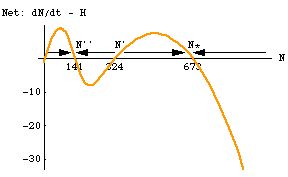
Puzzling lack of recovery? Check for sigmoid harvest function. Imagine a harvested population with a dN/dt and sigmoid harvest function like the one in Fig. 25.5. If a severe winter, epidemic or some other setback ever reduced the population below N' (324), it would decline to a new, lower stable point, N'' (141). Unless managers realized what the reason might be they might be puzzled as to why the harvested population simply wouldn't bounce back on its own. [The reduction would have to be driven by something other than the forces in our model. The model itself wouldn't allow the population to crash like that. It seems perfectly plausible though to imagine populations that spend 99% of their time governed largely by the forces modeled here -- logistic growth, a nonlinear harvest function -- but that could occasionally suffer catastrophes that aren't included in the model].
Fig. 25.6. Difference between dN/dt and H for the sigmoid harvest of Fig. 25.5. Note that net population growth (logistic prey growth minus sigmoid harvest) is positive in two different regions. Net growth is positive between N = 324 and N = 673, but negative above that point. This means that N* = 673 is a stable equilibrium point. Below N' = 324 the population declines, so N' is an unstable equilibrium. Below N = 141 the growth is again positive. This makes N'' = 141 a second stable equilibrium. If the population ever dips below N' it will settle on a new lower equilibrium, with lower N and lower harvest. Note also that the point of maximum net growth is actually in the lower positive region (at a prey number, N, of approximately 40).
Equivalence to the sigmoidal total response seen in Bay-breasted Warblers in Lecture 22. This is a different example of the possibility of multiple equilibria illustrated in Figures 22.1 to 22.4 of the first lecture on predation (Lecture 22). The sigmoidal predator response there also resulted in multiple equilibria (alternating between stable and unstable points). Look back at those notes and make sure you understand the conceptual link.
Note on population trajectory: remember, we are not dealing with phase plots here, so the vector sum approach is not what we do. Instead, we look at the impact of the difference between the functions (dN/dt - H) on N. If the sum is positive, N increases (you could put the rightward arrows right along the orange curve instead of along the X-axis). If the sum is negative, N decreases (you could put a leftward arrow along orange curve instead of along the X-axis).
Why not manage for a linear rather than a sigmoid harvest function, since the linear function doesn't have the multiple equilibria? The shape of the harvest function may not be something that the managers can really control. At the lower end, managers can't make people hunt, fish or commercially harvest if they simply don't think it's worth it for little reward. At the upper end, economics, a limited number of harvesters or some other factor may put a cap on the effort. The sigmoid harvest function may be more a fact of life than something one can easily manipulate. Of the three curves, it may be the most plausible -- and it can have the scary, puzzling consequence of an "irreversible" decline in the stable population size.
Points to ponder:
1) Alternating stable and unstable equilibria: I have already mentioned an interesting pattern that emerges when multiple equilibrium points exist. With multiple equilibrium points (such as here where the line squiggles back and forth across the zero line, and each crossing point is an equilibrium of zero net change) the system will alternate between stable and unstable equilibrium points. If you think about which way the arrows point, you will realize that this pattern is inevitable, At each crossing, the arrows will flip directions. That inevitably creates an alternation between stable (arrows point in to zero crossing) and unstable (arrows point away from zero crossing). Although it is not mathematically similar, a somewhat analogous alternation of effects occurs in some trophic interactions (look back at the sigmoid functional response curve and the coyote, scrubland bird examples of Lecture 21 and forward to the examples in Lecture 29 on regulation and trophic interactions).
2) Why might it be more likely that we would have
spruce budworm outbreaks (escape from regulation by predators) thanpermanent depression of the equilibrium population size (establishment of regulation by predators) of ungulates
by large predators (hunters, wolves)?
§§§§ §§§§§§§§§§§ §§§§§§§§§§§§§ §§§§§§§§§§§§§§ §§§§§§§§§§§§§ §§§§§§§§