Lecture 22 (Wed. 13-Mar-13) Introduction to predation

Return to Main Index page

Go to back to lecture 21  Mon. 11-Mar     Go forward to lecture 23 of Fr. 15-Mar

    Required reading:  Gotelli text, Chapter 6 (predation)
    Required reading: Saether. News & Views of Crooks paper (in WyoWeb folder)

What is predation?

I. Herbivory: eating plants; range from monophagy (eating just one thing) to polyphagy (eating many different types of food). The "phagy" part of the word refers to eating. For example, in cell biology, a phagocyte is a cell that "eats" other cells.

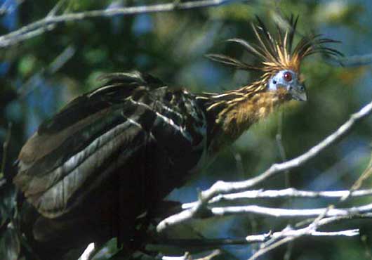
The hoatzin is a herbivorous bird of South America that uses a gut fermentation system very similar to that of cattle. 

II. Insect parasitoids: insects that lay eggs on or near host that is then consumed by the larvae. Likely to be at least somewhat specialized.

Ichneumonids are parasitoid wasps. They use the long ovipositor to lay their eggs in the hosts they parasitize.

III. Parasites: tapeworms, mistletoe, ticks. (Can also act as disease vectors for even smaller bacterial or viral parasites). Likely to be at least somewhat specialized -- often highly specialized.

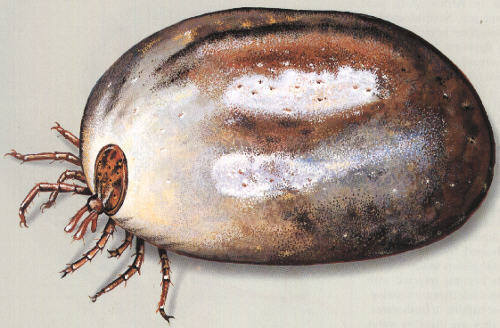
An ectoparasite (external), the tick Ixodes (which can carry Lyme disease).  Host-parasite interactions can have very interesting and complex dynamics. 

IV. Cannibalism: consumption of conspecifics.

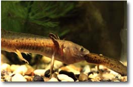
A cannibalistic salamander, eating a conspecific.  A small proportion of tiger salamanders, Ambystoma tigrinum, develop as cannibals, probably in response to crowding and lack of food resources.  They appear to avoid eating kin.  (Work of James Collins and David Pfennig)

V. Carnivory: "classic" predation, consumption of heterospecifics.  Lions and gazelles, flycatchers and insects, fish and aquatic prey; again, range from generalist to specialist. Long handling times lead to specialization, short handling times to broad diet.

Why does predation matter?

Predation can restrict the distribution of prey species or regulate their populations. We will see neat experimental evidence for how predators prevent vole cycles in a later lecture (Lecture 30).  That study, by Korpimakki and Norrdahl (1998), will be a required reading at that time.

Predation can act as a force to structure communities --

        Examples:

1)  Pisaster, a starfish, acts as a keystone predator whose presence or absence can change marine communities in major ways.  Ecologist Robert Paine showed that in the absence of Pisaster, a few competitive dominants (barnacles and mussels) can usurp all the space in the intertidal. Pisaster predation can free up areas of rock that can then be used by other species such as anemones.
            
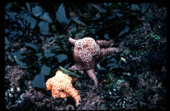
            Pisaster eating mussels and barnacles in the rocky intertidal. Photo from: http://life.bio.sunysb.edu/marinebio/rockyshore.html

2)  Sea otters reduce sea urchins and increase kelp -- difference in the nearshore community (water clarity and color) can be seen from space!  The kelp "forests", in turn, provide habitat complexity, prey refuges and spawning sites (e.g., for herring) that seems to increase the diversity of species that can exist in the nearshore environment. [Work of Jim Estes, UC-Santa Cruz]
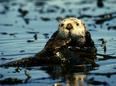             Sea otters can cause major changes in shoreline communities by reducing sea urchins and allowing kelp growth
The prevailing idea (not without its critics) is that such keystone predators can maintain species diversity by preventing the dominance of one or a few species (the mussels in the Pisaster case, the urchins in the otter case).

Trophic cascades: changes in abundance of top predators can have major impacts on species two or three trophic levels below them.  One example is the interaction between wolves, moose and trees on Isle Royale in Lake Superior (McLaren and Peterson, 1993).  That will be an assigned reading when we get to the section on population regulation (approximately Lecture 29) but it wouldn't hurt to read it now.

Predation as an important mechanism of natural selection -- predation has been suggested as a major influence on phenomena as disparate as evolution of warning colors and mimicry, cost/benefit balances in sexual selection (look back at the guppy coloration example I gave in Lecture 2), tendency to flock or herd, life history evolution (age of first breeding, nesting strategies), and anti-predation adaptations/the "unprofitable prey" hypothesis (stotting behavior in ungulates or bright coloration in some birds may act as a signal that the prey are not worth chasing -- essentially a signal from the prey "I see you, so don't bother chasing me"). [See, for example, Götmark, 1995].

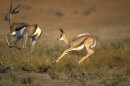Stotting is a peculiar four-legged hopping gait used by a variety of prey that acts as a signal to deter pursuit by predators.  In studies of African gazelles, Caro found that mortality risk was significantly lower for prey that had stotted. 

Indirect effects of predation on behavior may be more important than direct effects through mortality-- several possible ways exist that predators can have major effects on prey populations by changing prey behavior rather than by actually killing them. 

1. Vigilance -- prey may spend more time being vigilant (scanning for predators) and therefore less time feeding.  As a result, many individuals (not just the relatively few eaten) may be in poor condition, lowering their survival or fertility. 
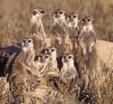            Meerkats scanning for predators

2. Habitat selection -- prey may shift from preferred to marginal habitats, again having a population-wide effect on condition.
           Example: Elk may move from risky but food-rich open environments to safer but food-poor forested environments.

3. Grouping -- predation pressure may select for herding, schooling or grouping, again with possible population-wide effects on foraging rates and condition.
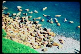              Male walrus crowded together on a beach in Alaska (for predator avoidance)

4. Inducible defenses -- predation pressure may cause prey to produce defensive features such as spines or toxins. 
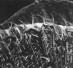            Bryozoans exhibit spines in the presence of potential predators (from life.bio.sunysb.edu/.../shallowsubtidal.html)
When the bryozoan Membranipora membranacea encounters a predator such as the sea slug Doridella steinbergae it grows protective spines near the periphery of the colony. This shot is a closeup of the edge of a colony. Drew Harvell has found that although the spines defend against the predator, they encumber a cost and overall colony growth is reduced. Thus it is valuable to have this defense "programmed" only when predators are encountered. Otherwise the colony will grow faster and presumably also reach a reproductive size sooner.

Ecological release of mesopredators in California sage scrublands.

Crooks and Soulé (1999) examined the bird populations of patches of sage-scrub habitat in southern California.  What they found was that the presence or absence of large predators (in this case, coyotes) had a major impact on the population dynamics of birds.  In the absence of coyotes, mesopredators (medium-sized predators including striped skunks, raccoons, gray fox, domestic cat and opossum) increased in abundance and depressed the abundance of native birds, often to the point where local extinctions occurred or were inevitable.  Thus, the fate of the birds is driven largely by that of a predator two trophic levels above it.  If the factors that limit a population are removed, the population may experience what is called ecological release.  How does this resemble the character release we analyzed with Galapagos finches in  Lecture 19 webnotes on competition?  Both involve the absence of a biotic interaction (competitor or predator) and result in a response in a niche dimension (shown by the change of bill morphology in the Galapagos finches) or in population size (in the case of mesopredators released from control by a higher predator). [The original Nature paper by Crooks and Soulé and the accompanying News & Views article by Bernt-Erik Saether will be in the WyoWeb folder as strongly recommended readings].

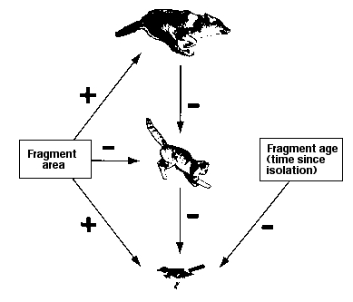
Fig. 22.5.  Schematic outline of interacting effects of fragmentation, large predators and mesopredators on bird populations.
1)  Fragment area has a positive effect (+ arrows on left) on  coyote and scrubland bird populations.  That is, larger fragments have a positive effect on coyotes and birds.  Fragment area has a negative effect on mesopredators (- arrow to cat) -- there are fewer in large fragments.
2) Coyotes have a negative effect on mesopredators (more coyotes, fewer cats).
3) Mesopredators (such as cats) have a negative effect on birds.
4) The longer a fragment has been isolated (disconnected by intervening urban or suburban development) the worse the decline of bird populations.
Working together, these factors (small fragments, long term isolation and high numbers of domestic cats and other mesopredators) mean that many scrub fragments have almost no chance of supporting viable populations of native scrubland birds such as Western Scrub-Jays, California Quail, California Gnatcatchers, Wrentits and Bewick's Wrens.

Major message:  loss of the top predator (coyote) leads to "ecological release" of mesopredators such as cats that then decimate the native bird populations.

Using multiple regression to do the closest possible thing to an experiment.  How important is the absence of the predator?  That is, might it be that the mesopredators simply do better in the small fragments?  Crooks and Soulé checked that by checking coyote presence while holding other factors constant.   That is, did simple presence of coyotes (even in fragments of the same size and age) decrease mesopredator abundance?  YES.  Crooks and Soulé assessed coyote presence by using a combination of track indices and remotely triggered cameras.  Fragments with higher coyote visitation had fewer mesopredators and more songbirds.

How did coyote abundance and presence affect mesopredator abundance?

1) Mesopredators avoided fragments where coyotes were present.
        a) Perhaps the most interesting way that this worked was that cat-owners kept their cats indoors in places where coyotes were known or suspected to occur.
        b) Even within a particular patch, mesopredators were less common in three-month periods where coyotes were present than in three-month periods where coyotes were absent. Thus, mesopredators avoided coyotes temporally as well as spatially.

2) Coyotes directly killed mesopredators. 21% of coyote scats contained cat remains. 25% of radio-collared cats were killed by coyotes.

Why are domestic cats the most important and detrimental mesopredators?

    1) Cats are recreational hunters maintained at far above the carrying capacity of the scrub fragments they hunt in. A fragment of approximately 20 hectares could support 35 cats from surrounding developments -- compared to just one or two pairs of native foxes that are not subsidized.

    2) A fragment surrounded by 100 or so houses could result in cat capture of 840 rodents, 525 birds and 595 lizards per year. These levels of "harvest" are almost certainly unsustainable.

Trophic level interactions

    The interaction between the birds and the coyotes is indirect -- via the effect of the coyotes (top predator) on the trophic level below them (the mesopredators) that in turn determine the abundance of the lowest trophic level considered here (the birds).

Questions to ponder:

What would you predict for the influence of the presence or absence of coyotes on the trophic level below the birds?

What would you predict for the influence of a predator above the coyotes (such as wolves or bears)?

If you had all the money and resources you needed, what experiments might you design to follow up on the study by Crooks and Soulé?

Functional and numerical response by predators

Holling (1965) developed an important concept in predator-prey dynamics -- the idea of functional (eat more prey) and numerical (produce more baby predators) responses by predators to increasing prey.  Murdoch (1977) expanded this concept by adding two more responses: aggregative (clustering of predators in an area where prey have become more abundant) or developmental (increase or decrease consumption as the prey mature).  We will focus on some lessons to be learned from the combination of functional and numerical responses.

We will explore the synergy of a functional and a numerical response with the classic example of the interaction between the Bay-breasted Warbler, Dendroica castanea, and the spruce budworm, Choristoneura fumiferana.   Most years, spruce budworm occur at relatively low densities in the boreal forests of Canada, as do the Bay-breasted Warblers that feed on them.  Occasionally, though, the budworms irrupt in massive numbers.  Although the warblers also increase greatly and feed voraciously on the budworms, they simply can't keep up with the explosion and the budworms can cause massive damage to large areas of forest.

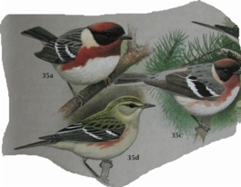
Bay-breasted Warblers, which breed in boreal forests and which respond to increases in spruce budworm both functionally and numerically.  At low densities of budworms, the warblers can keep the budworms in check, but above a threshold density, the budworms irrupt and can cause massive damage to trees.

Holling described three types of functional response: linear, hyperbolic and sigmoidal

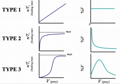
Figure 22.1. Three types of functional response: linear, hyperbolic and sigmoidal.

The graph on the right depicts proportion of the Victim population (V) consumed.  We will work with a sigmoidal response here, but go to a simpler linear functional response when we develop the Lotka-Volterra predator-prey models in the next lecture. 

How does this "escape from predation" occur?

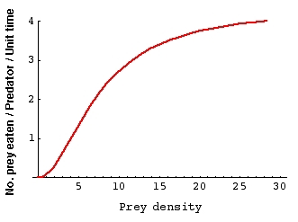
Fig. 22.1a Sigmoidal functional response.  The functional response measures how many budworm prey the warbler predators eat (as a function of prey density).  Notice the units for the Y-axis (No. prey eaten / Predator / Unit time ). Notice also that for prey densities above 10 (meaning 10 larvae per square meter of foliage), the predators no longer increase their consumption.  They have a maximum rate probably determined by their handling rate.
{Data derived from a mixture of Hassell (1981) and Mook (1963) via Krebs (1994)}.

 

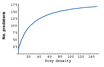
Fig. 22.2 Numerical response.  Notice the units for the Y-axis (No. of predators).  Notice also that, at high densities of prey, the number of predators levels off (factors other than prey availability may keep them in check).

 

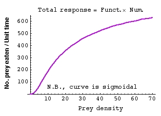
Fig. 22.3. The total response, calculated by multiplying together the equations for the functional and numerical responses. Notice the units for the Y-axis (multiply out the units of Figs. 22.1 and 22.2 to see how this works out).  Note that the curve is now sigmoidal (the inflection point is squashed down in the bottom left-hand corner -- this is sigmoidal but not symmetric at half the asymptote like the logistic). The sigmoid shape arises if either the functional response is sigmoidal or if both the functional and numerical  are hyperbolic (smooth upward curve that flattens out, like the numerical response in Fig. 22.2). We will come back to the consequences for sigmoidal predation curves when we consider the problem of harvest (a specialized form of predation).

 

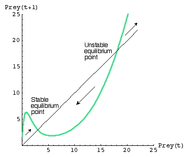
Fig. 22.4.  One-dimensional map (like those used for the discrete logistic) for a predator-prey system where the total response is sigmoidal (as in Fig. 22.3).  The map allows us to calculate the density of Prey at time t+1, given the density at time t.
Note that the map crosses the line of equality [ Prey(t+1) = Prey(t) ] at two places.  That means we have TWO equilibrium points.  The lower one is stable, the upper one unstable.  Wherever the map (green line) is above the line-of-equality, the prey are increasing. Wherever the green line is below the line-of-equality the prey are decreasing. At any density below about 19 larvae per square meter of foliage, the prey will move towards a stable equilibrium of approximately 3/m².  That is, at spruce budworm densities of 3 to 19/m² the warblers keep the budworms in check (drive them back down to a density of 3/m²).  If, however, the budworms increase suddenly to densities greater than 19/m² (which they do occasionally because they have a very high intrinsic rate of increase) they "escape" regulation by the predator.
We will see similar alternative states in the harvest lecture (Lecture 25).

The equation that generates the 1D map in Fig. 22.4 is:

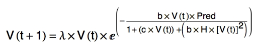             Eqn 22.1

In Homework 6, we will work with values for Eqn 22.1 to generate a 1D map like the one shown above, as well as to track the trajectory of population densities from different initial densities. You are not responsible for knowing much about the equation.  You should, however, be comfortable with interpreting a 1D map like the one in Fig. 22.4, and should understand the trajectories that will result from different initial population densities. 

How do the two equilibrium points here differ from what we found with the discrete logistic in Lectures 16 and 17?  Look back at Figs. 17.1 through 17.4.  There, the map lines crossed the black 45° slope line-of-equality only once (always at K).  That single crossing was either a stable equilibrium point (when r < 2) or unstable (when r > 2).  Here we have two crossings -- leading to one unstable and one stable point. We will return to alternation of stable and unstable equilibrium points in Lecture 23 (harvest). 

Major conclusions:

If the total response is sigmoidal then:

1) For a certain range of prey densities, the predator can keep the prey "in check".
2) At high prey densities, the prey can "escape" the check on growth provided by the predator. From there on, its own density-dependent controls will have to kick in to keep the population from irrupting.

Questions to ponder:

1)  Is it likely that wolves, hunters or other large predators keep ungulate populations at low densities?  Or is it more likely that most ungulate populations exist at high enough densities that they are controlled largely by their own logistic population dynamics (density-dependent regulation produced by crowding)?  What is happening in some places in the eastern United States with deer populations in the absence of large predators and of hunting?

2)  The green line may cross the line-of-equality again at some higher prey density.  Will that be a stable or unstable equilibrium?  What might happen, though, after a huge irruption of spruce budworms that devastates the forest habitat?  Look back at Lecture 5 and Lecture 2 for ideas.

Crooks, K.R., and M.E. Soulé. 1999. Mesopredator release and avifaunal extinctions in a fragmented system. Nature 400: 563-566.
                 A strongly recommended reading, available in the WyoWeb folder.

Götmark, F. 1995. Black-and-white plumage in male pied flycatchers (Ficedula hypoleuca) reduces the risk of predation from sparrowhawks (Accipiter nisus) during the breeding season. Behav. Ecol. 6: 22-26.

Hassell, M.P. 1981. Arthropod Predator-prey Systems. Princeton University Press, Princeton, N.J.

Holling, C.S. 1965. The functional response of predators to prey density and its role in mimicry and population regulation. Mem. Entomol. Soc. Can. No. 45.

Korpimäki, E., and K. Norrdahl. 1998. Experimental reduction of predators reverses the crash phase of small-rodent cycles.
Ecology 79: 2448-2455.

Krebs, C,J. 1994. Ecology: The Experimental Analysis of Distribution and Abundance. 4th Edn. Addison-Wesley, Menlo Park, CA.

McLaren, B.E., and R.O. Peterson. 1994. Wolves, moose, and tree-rings on Isle Royale. Science 266: 1555-1558.

Mook, L.J. 1963. Birds and the spruce budworm. Pp. 268-271 In The Dynamics of Epidemic Spruce Budworm Populations (R.F. Morris, ed.). Memoirs of the Entomological Society of Canada, No. 31.

Murdoch, W.W. 1977. Stabilizing effects of spatial heterogeneity in predator-prey systems. Theoretical Population Biology 11: 252-273.

Saether, B.-E. 1999. Top dogs maintain diversity. Nature 400: 510-511. A required reading, available in the WyoWeb folder. (This is a News & Views overview of the Crooks and Soulé paper.  News & Views overviews give a less technical overview of the main points of a scientific paper.  It often helps to read that before you read the original paper).

Return to top of page                       Go to forward to lecture 23 of Fr. 15-Mar