Inflection of the logistic; asymmetric Gompertz curve;
    Populations: definitions, characteristics, processes, and limits

Suggested reading: Wells and Richmond, Populations, metapopulations and species populations (in WyoWeb folder)

Return to Index page       Go back to notes for Lecture 5, 25-Jan     Go forward to notes for Lecture 7,  30-Jan

Go to web page for dispersion and Poisson related to Homework # 2.

Last time I introduced the logistic equation for population growth and illustrated how we can use logarithmic transformation to linearize the equation, so that we can estimate r from a plot of empirical data.  Today I will use the derivative method to find the inflection point and then briefly mention an alternative "bounded growth" model, the Gompertz curve, which has the (sometimes desirable) property of being asymmetrical about the inflection point.  [Asymmetrical means non-symmetrical -- i.e., that the shape is different on each side of a dividing line.  Radial symmetry, for example, means that an object such as a sea urchin is symmetrical around a line from pole to pole].  Then I will turn to definitions, characteristics and limits of populations.

Scared by the calculus?  I will not use calculus all that much in this course.  I do though, encourage those of you that haven't had it, or are very rusty to get some sort of primer on basic techniques.  I will put some excerpts from at least one good brief intro. into the suggested reading packet in the Science Library.  Understanding derivatives is probably the single most important thing (e.g., first derivative as the slope and second derivative as the acceleration).

It is obvious by inspection that the logistic curve is concave up at the beginning and concave down at the end. Where does the shape change? This is called the inflection point. Mathematically, the inflection point is where the acceleration (second derivative) switches from positive to negative. That is, the acceleration (second derivative) = 0.  The logistic, as normally plotted (e.g., Fig. 5.1 or 6.2), shows population size as a function of time and has a sigmoid curve.  Its slope would be the rise over the run or dN/dt.  We already have that (Eqn 5.1), so all we need to do is take the derivative of our Eqn for dN/dt to find the inflection point.  Let's begin by rearranging Eqn 5.1 (multiplying out to get terms in N² and N) to get it in the form:

                                                                    (Eqn 6.1)

The graph of Eqn 6.1 (plotting population growth on the Y-axis as a function of population size on the X-axis) is shown in Fig. 6.1.  Now take the derivative of Eqn 6.1 with respect to N and set it to 0.   [Setting derivatives to zero and then finding parameter values is a key technique that recurs repeatedly in population ecology approaches -- we will use it for stability analyses, finding the maximum or minimum point on a curve, and for finding inflection points].

Reminder of how to do a derivative for power functions:

                             derivative of cx^a = acx^a-1

The derivative of a constant times the quantity "[x to the power of a]" is the exponent (a) times the constant (c) times the inside-the-brackets-quantity "[x to the power of a-1]". Remember also that anything to the zero^th power is 1 (so rN^1-1 = rN⁰ = rX1 = r).  Applying that to the RHS (= "Right-Hand Side", a term I will use repeatedly) of Eqn 6.1 and setting the LHS (left-hand side) to zero gives us:

                                  (Eqn 6.2)

The last thing on the right is the first derivative of Eqn 6.1.  Now move the r over to the left and divide both sides by -r to get:

                                                                                                               (Eqn 6.3)

A final rearrangement yields:

                                                                                                               (Eqn 6.4)

Voila! The inflection point occurs at half the carrying capacity.

Note also that if we plot dN/dt as a function of N,as in Fig. 6.1, we get a humped curve that is symmetrical around the midpoint (K/2). That means the growth rate is highest at the inflection point. We can see the "acceleration" changing directions -- the slope of the sigmoid curve of Fig. 5.1 reaches its maximum at K/2 and then declines from there. At K, the slope of Fig. 5.1 (the sigmoid curve at the beginning of the previous lecture) is flat (slope = 0).

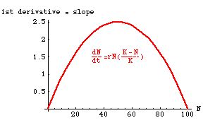
Fig. 6.1.  Growth rate (dN/dt) as a function of population size (N) for a population with K=100.  Note that the growth rate peaks at N = K/2 = 50 and is symmetrical around it.  This plot makes it easier to see that the inflection point is where the "acceleration" changes from increasing to decreasing.  That is, the second derivative is zero at the top of the hump.
Note that there are two places at which the population is not growing  --
      1) when N = 0
      2) when N = K.
In between those two zero points, N is < K, so the equation will be a positive number, meaning that it pretty much HAS to have the humped shape shown.
• Questions to ponder:
1) For this example,  dN/ dt has a maximum at 2.5; what is the value of r?
2) We can take one more derivative: if we take the derivative of the expression at the right of Eqn 6.2, what do we get and what does it tell us about the acceleration of dN/dt?
3) What would a plot of the per capita logistic growth rate look like?

The logistic is symmetrical about this inflection point. Some populations, however, begin to show strong negative effects of crowding well before they are at half the carrying capacity. A function that permits us to have an asymmetric sigmoid curve is the Gompertz function. The equation is a slightly intimidating set of double exponentials:

                                                                                         (Eqn 6.5)

You won't need to memorize this formula, I just want you to be aware that a method exists for modeling asymmetrical sigmoid population growth.  I may expect that you remember that the name "Gompertz" is associated with this sort of asymmetric, bounded growth.

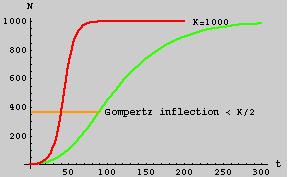
Fig. 6.2. The Gompertz curve (green) for population size (N, on the Y-axis)
as a function of time (t, on the X-axis).  For comparison, a logistic curve,
with the same parameters (same K, same r), is shown in red.
Note that the Gompertz curve is asymmetrical, with an inflection point < K/2
(it happens to be at K/e = 367.8, and is marked by the brownish line).
The inflection point of the logistic is at K/2 = 500 as derived in Eqns 6.1 to 6.4.

In the last few lectures we have examined two basic models for growth of single populations -- exponential and logistic.  Now, we will ask the question: what is a population?  Then we will look at some characteristics and processes that are important in studying populations and consider some general ways in which populations interact with their environments.

Population is the level of biological organization we are interested in

                                                                                           population
                    {vs. biome, ecosystem, community, species,                     , individual, organ, cell}.

The levels above and below population are characterized by distinct "boundaries".  It is pretty easy to tell where you start and your classmate ends.  Likewise, species "tend" to be sharply bounded in most cases.  Ornithologists have little trouble telling a mallard from a pintail,  ichthyologists have little trouble telling a cutthroat from a brown trout, etc.  Except at hybrid zones, distinct gaps exist between species.  With populations, however, it can be harder to decide on a satisfactory boundary.  If we are in a white spruce forest in northern Canada, what is the population boundary of the spruce around us?  The spruce stretch in an essentially unbroken swath from the Atlantic to the Pacific.  Surely we don't want to consider all of them as constituting the same population.  In other cases, sharp habitat boundaries may make our task relatively easy.  The population of pikas in the Snowy Range to our west is fairly well separated from the next nearest population in the Front Range of Colorado.

Let's leave the boundary issue in the back of our minds for a moment, while we consider various different definitions:

Krebs (1994, p. 151) "A group of organisms of the same species occupying a particular space at a particular time".

Particular space — suggests delimited geographically.
Particular time — changes over time — dynamic. Another definition of population: Cole (1957)  "A biological unit at the level of ecological integration where it is meaningful to speak of birth rate, death rate, sex ratios and age structures in describing properties or parameters of the unit. These processes occur at the level of the individual, but have emergent properties at the level of the population."

Wells and Richmond (1995) suggest that populations must be disjunct in one of three possible ways:

Spatially                          (almost always a prerequisite for the remaining two)
Genetically                      (population geneticist's emphasis)
Demographically            [Cole's (1957) emphasis]

Biologist must define a population in a biologically useful manner. Political boundaries, for example, usually are not biologically meaningful (but may sometimes be a necessary factor impinging on biological decisions).

A population is a biological unit that fluctuates in size and composition. Population dynamics is the study of how the composition changes over time (abundance, density, sex ratio).

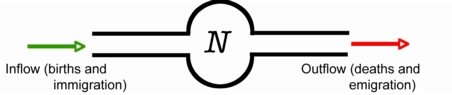
Analogy: Reservoir = population dynamics — both are dynamic systems for which it is appropriate to the study of rates of "intrinsic" or endogenous input and output (birth/deaths = flow in from and out to a connected river), vs. "extrinsic" or exogenous input (immigration = rainfall) or output (emigration = evaporation). What is important about the analogy?  Both systems are dynamic (change over time), both depend heavily on various kinds of rate-based processes (births per individual per year; rainfall per acre per year), and each can be characterized as having inputs and outputs both from "within" the system and from "outside" the system.

Fluctuations in populations are driven by a suite of processes that include: interactions between members of population, interactions between different populations, or interactions between populations and their environments.

Population characteristics, and processes; interactions with the environment

Processes: (forces that can actually drive population changes)
     (we have examined simple growth consequences of the first two)

Birth
Death

Immigration
Emigration

Processes that involve aspects of the environment

Competition (intra- and inter-)
Predation
Disease

Characteristics:  (attributes or parameters, not driving forces, though they may have consequences that will cause change)

Size: (indices vs. enumeration) Census (complete count of all the individuals)
Density
Structure: Age (matrix models particularly useful for assessing age structure & consequences)
Sex ratio
Genetic
Physiological or developmental state
Dispersion: uniform, random, clumped (we will later look at ways to assess dispersion quantitatively)

 

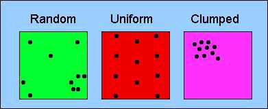
Figure 6.3.  Three major patterns of dispersion.  Random dispersion is essentially the "null model" -- the pattern we might expect if no special forces were acting on the spatial distribution of individuals in the population.  Examples of uniform dispersion can result from behavior (e.g., territoriality) or allelopathy (production of toxins that keep others from establishing nearby in plants).  Clumped distributions can result, for example, from aggregative behavior (herding or schooling) or from restricted availability of suitable habitat or microhabitat.  The relationship between the variance and the mean of neighbor-neighbor distances is a key parameter in the quantitative analysis of spatial dispersion.
Go to web page for dispersion and Poisson related to Homework # 2.
   The Poisson distribution has many other applications in biology. Just for example, it is used to describe
     1) the expected number of offspring per family in calculations for captive breeding management;
    2) whether the timing of breeding is spread out or clumped in time (Marsden et al. 2004)

Interactions with the environment: (features outside the population that can influence it in fundamental ways)

Food
Cover
Weather
Special needs (nest sites, mutualist partners)

These three aspects (population processes, population characteristics and environment) can interact in very complex ways to produce the dynamic patterns of population ecology. Our job is to understand some of the most important interactions and how they should work from a theoretical and empirical basis. If you understand the processes that drive population dynamics, you can make progress towards prediction of future fluctuations.

The first step in making statements or predictions about populations is to delimit them. Appropriate scale will depend upon dispersion (see Fig. 3.1) and natural history/mobility.

What we desire to describe or predict about population will influence where we set boundaries

If the animal is sedentary and we want to estimate density, any boundary with reasonable number appropriate

If animals are mobile — small units can present problems (too much interaction with surrounding conspecifics, problems of sample size for estimation).

Examples:

Sedentary -- Barnacles (or plants) -- any plot that contains a fairly large number
(50, 100, 200) will work.   The plot might safely be as small as 10 meters X 10 meters.

Mobile -- Wyoming elk herd -- if we pick just a few square kilometers they may be there so rarely that we will not have good counts, replication etc.

In population genetics, Wright (1946) provided an "artificial" but useful delimiter for a population by defining a "neighborhood size," N_e, given by the formula:

N_e = 4 ps²d                                                                                                    (Eqn 6.6)

where p (pi) indicates that we are discussing a circular range, the s² (sigma-squared) is the variance in the dispersal distance, and d (delta) is the density.  [Note: it is very helpful always to keep an eye on the units.  Here we have two "pure numbers" (4 and p), density, d, as number per area (e.g., m²) and the variance of dispersal as squared distance units (e.g., m²).  The squared units cancel.  The end result is a number of animals, as it should be].   The idea of this neighborhood size is to delimit an area within which individuals can be assumed to mate at random.  We will explore this equation for neighborhood size in Homework 2. 

References:

Cole, L.C. 1957. Sketches of general and comparative demography. Cold Spring Harbor Symp. Quant. Biol. 22: 1-15.
        Reprinted in Tamarin, R.H. (ed.). Population Regulation. 1978. Dowden, Hutching & Ross, NY.
Krebs, C.J. 1994. Ecology: The Experimental Analysis of Distribution and Abundance (4^th ed.). Addison-Wesley, NY.
Marsden, A.D., and K.L. Evans. 2004. Synchrony, asynchrony and temporally random mating: a new method for analyzing
            breeding synchrony. Behavioral Ecology 15: 699-700.
Wells, J.V., and M.E. Richmond. 1995. Populations, metapopulations, and species populations:
            what are they and who should care? Wildl. Soc. Bull. 23: 458-462. (on WyoWeb)
Wright, S. 1946.  Isolation by distance under diverse systems of mating. Genetics 31: 39-59. 

§§§§§§§§§§§§§§§§§§§§§§§§§§§§§§§§§§§§§§§§§§§§§§§§§§§§§§§§§§§§§§§

Return to top of page         Go forward to notes for Lecture 7,  30-Jan