Lecture 7 (30-Jan-13)

Dynamic changes in populations

(Population estimation: indices vs. absolute density)
            (N.B., this is web-only material; you are responsible for it)

Return to Index page          Go back to notes for Lecture 6.  28-Jan      Go forward to notes for Lecture 8,  1-Feb

               Go to optional web page with greater detail on Line Transect estimation (and Mark-Recapture)

Examples of dynamic population patterns

   Changes within a population (intrinsic or endogenous)

       • Change in sex ratio: increase in females may lead to increase in birth rate if constraints on female offspring production limit growth.

E.g., much of the practice of big game harvest is predicated on the idea of female demographic dominance. Since one male can inseminate many females, we can harvest a high proportion of males without really impacting population growth (in fact may enhance it, by decreasing intra-specific competition).

       • Change in age ratio: increase in age class with highest reproductive value leads to increase in birth rate.

• Change in density: can change reproductive success, survival rates or probability of dispersal. High density generally results in depressed birth rate or increased death rate (or increased emigration). Low density can also result in depressed birth rate or increased death rate (this is known as the Allee effect -- for example, at low densities individuals might have a hard time finding mates, or they might lose a predation-avoidance benefit of herding). This is sometimes called positive density dependence -- that is, as density increases, the effect is a positive one on the population growth rate.  That is what is happening in the left-hand part of the curve below.  The right-hand side shows negative density dependence (as N increases beyond 50, the birth rate starts to drop). 

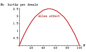
Fig. 7.1.  The Allee effect, whereby vital rates (such as births or survival) are depressed
when N is low.  Note that for this example we have a peak of fertility at intermediate
population size.  The reduction at high densities is more expectable and is incorporated
in the concept of a crowding effect or carrying capacity.  This curve looks very much like that of Fig. 6.1,
but has different units for the response variable (Y-axis has births/female rather than dN/dt).
[Compare to the per capita plot of dN/dt in Fig. 6.1]

   Changes between populations (extrinsic or external)

• Predator/prey interactions Example: when their primary prey (hares & lemmings) are at low densities, foxes may shift their attention to ptarmigan or geese. This predator shift can have dramatic impacts on the nest success of the birds (the 'alternative' prey), particularly when fox densities are still high after a lemming peak. Predator-prey interactions in 'simple' communities are particularly susceptible to time lags.

• Interspecific competition -- competition between species for limited resources may have significant effects on population dynamics.

Interactions between population & environment

• Weather:
       If the weather in the fall is cold wet before snowfall, red-backed vole production will decrease.
       Drought in prairie potholes may greatly depress duck production

• Habitat features:
        A forest with very few snags may lead to fewer Pileated Woodpecker cavities and thereby lead to fewer sites
             for secondary cavity users such as flying squirrels, small owls, and many birds.
       Timber harvest and road construction may cause increased runoff and
            siltation of streams, and thereby compromise salmon spawning.

An understanding of population ecology can be directly useful for wildlife management largely because it is predictive.

Examples:

Harvested species: help maximize harvest while minimizing 'risk' of crash

Control of harmful species: allows assessment of costs and benefits -- predator 'control' may actually have the completely unintended consequence of maximizing population growth rate and turnover.

Endangered and rare species: evaluate risks (persistence times) and model alternatives for management.
1)  Two European researchers used a sensitivity approach (and reproductive values) to help managers decide which age class of animals to reintroduce. They suggested that despite some loss, reintroducing adult rather than juvenile individuals to the wild from captive breeding programs made sense for two species they analyzed (an ungulate and a large bird).
2) Knowing the assumptions and limitations of matrix-based demographic projection models could help managers decide which parts of the life cycle are amenable to management (e.g., increasing fledgling survival) and how much effect those changes might have.

Nongame wildlife:Marquis and Whelan (1994) studied the effect of insectivorous birds on vegetative damage by insects.   They excluded neotropical migrant songbirds (insectivores) from oak trees and demonstrated significant decrease in tree growth (because caterpillars and other herbivores increased).  Their results suggest that songbirds have a strong, if indirect, effect on timber productivity.  That study was replicated in Panama (tropical forest), and to the surprise of many ecologists, produced a similar effect there.  A recent study by Kalka et al. (2008) found that bats may play an unexpectedly large role in the tropical effect of excluding herbivores. [The Marquis and Whelan paper will be a required reading later in the course, but reading it first now would not hurt].

Marquis, R.J., and C.J. Whelan. 1994. Insectivorous birds increase plant growth through their impact on herbivore communities of white oak.  Ecology 75:2007-2014.
Kalka, M.B., A.R. Smith, and E.K.V. Kalko. 2008. Bats limit arthropods and herbivory in a tropical forest. Science 320: 71.

Note: the rest of this "lecture" is web-only material.  

Sometimes, though, the pressing practical need is to count individuals or to estimate trends in population size.  Next, we'll look at population estimation -- mostly ways of assessing fluctuations in abundance and survival.  Dr. Merav Ben-David, who teaches the Game Management course (ZOO 4300) covers that extensively in her course, so I will touch only briefly on these estimation techniques.  Because this course is largely concerned with principles, processes and theory, and because the material on estimation is fairly straightforward,  I am not going to cover the estimation and line transect material in lecture.  You are nevertheless responsible for everything that is in these web notes.

Population estimation: demographic rates and estimates of density

Population estimation: things we will be very interested in estimating include survival (e.g., the P_i for Leslie matrices), productivity (the m_i of an l_xm_x schedule) and abundance (relative or absolute measures of density).

The most challenging estimation problems tend to be associated with abundance and survival. It tends to be relatively easier to get accurate measures of reproductive output (easier to count eggs, fawns, etc. than to assess survival rates). Our first look will be to look at estimating abundance with the fundamental dichotomy between indices (relative abundance) vs. censuses (enumeration, absolute density).

Examine the dichotomous key to assessing population abundance over time or space that is in the WyoWeb folder.
(You will also receive a single page version as a handout in class )

A note on time scale: the very first question asks us about whether the population is closed.  No population can be closed and continue to persist.  So.. the key words are 'during the census'.  On a 5-year time scale a Sage Grouse population will almost certainly be open, but if we can get in there and do our sampling in a few weeks in the fall it is probably safe to assume the population is closed 'during the census'. We can repeat the closed-population technique several or many times during the course of a long study -- what matters is the per-census time scale, not the time scale of the study as a whole.

If we are going to use an index (the Method 1, of the dichotomous key), we seek one that has a linear relationship to population number or density -- that is, more of the thing we can measure easily (such as tracks or scat) indicates more of the animals whose abundance we are trying to estimate.

Examples (plus the linearity expectation)

Mt. lion tracks per unit of aerial transect (more tracks = more cats)
Mice captured per trap night (more captures = more mice)
Eggs per meter of spawning substrate (more eggs = more recruitment)
Dove coo counts (more coos = more doves)
Elk calves per monitored unit (more calves = more harvestable)

Advantages of indices:

Efficient: lots of data gathered per unit effort.
Good for extensive preliminary studies: can cover large areas
Detect changes in abundance over temporal or spatial scales
It won't tell us absolute density but it will tell us about trends in space or time

Disadvantages of indices:

Detectability may vary with:
Time of day
Season
Weather
Vegetation
Terrain
Observer

Indices (and counts) require validation and examination of potential biases

One example of a lack of linear relationship was pointed out by Rotella and Ratti (1986) in JWM.
Calling frequency of gray partridges in the morning was highly correlated with density (r = 0.955).
        Evening calling was not. Morning calls therefore meet the linearity assumption, evening calls would not.
Require multiple replicates to reduce variance of estimate Replication is a fundamental aspect of scientific analysis -- it is extremely important in experimental design, for example. Also very important in any of the estimation techniques we will consider.

How can we convert indices to estimates?

Randomly sample from within the sampling design of the index and do valid measurements of absolute density. Then regress enumeration/census on index.   Eberhardt and Simmons (1987).

Advantages of counts/censuses that measure absolute density: May be the necessary input for some management considerations, for studying competition, or for exploring predator-prey interactions

TOTAL COUNTS (over entire area) ideal but usually not feasible. Some exceptions where counts are feasible:

Tawny Owls in Britain - highly territorial, stationary populations, vocal, long lived
Scrub-Jays in Florida; complete monthly census of all banded birds on approximately 50 territories
                (Woolfenden and Fitzpatrick, 1984).
Electrofishing, or poisoning with Rotenone
Pupfish in small pools
Radio-collar one animal per pack and then locate wolf packs
Systematically traverse an area-- drive counts of deer in MI
Aerial surveys of manatees in FL

We will now follow one particular path in the dichotomous key:
      Absolute density required? YES.
              Feasible to count all in study area? NO
                   Capture or count more appropriate? COUNT
                           Is population dense? YES

a. Spot mapping birds
       Grid with/ flags or stakes. 25 m transects + 25 m grid lines
       2-10 ha plot
       Replicate 7-10 times
       Plot locations of singing males on maps (especially simultaneous song)

Disadvantages:
      Problem defining territory
      Time intensive
      Boundary conditions (hard to definitively delineate boundaries;
             hard to ensure that males seen or heard are correctly assigned to presumed territory)

b. Total counts on sample plots (used for assessing vegetation cover in habitat studies)

Quadrats Examples: bald eagle nests, colonial seabird counts at colonies
Assumption: none missed, common, best if immobile (e.g., plants, nests)
Scale problems: small deer pellet counts may overestimate density by factor of 5.
Object/animal in or out of plot?
     Observers may be tempted to record it as being in when actually out but very close to boundary.
Shape: circle has minimum boundary

Rectangle gives better variance estimate (improved precision) Boundary bias:  For any square plot, the boundary of disconnected square plots vs. connected will be X times as large, where X is the number of subsquares. So, if we have a 25 square plots vs. a single 5X5 plot, the perimeter of the disconnected plots will be 5 times as great as that of the contiguous plot. For a 4X4 plot the factor would be 4, etc. That means that any boundary problems could get huge if we have a large number of disconnected subplots vs. large single plots. Take-home message: If we have too many small plots we may run into biases or other boundary-related problems.

Let's follow another path in the dichotomous key:

Absolute density? YES.
       Count all in study area? NO
                Capture or count? COUNT
                            Is population dense? NO
                                      Can all animals be detected at a distance? YES

c. Strip transects

Tradeoffs

If it's too narrow, very few observations and high variance (low precision)
If it's too wide, bias because some doubt as to whether all objects detected.

Tradeoff between bias in wide strip (unknown number missed) and precision in narrow strip (very few animals seen per strip, so number will vary from time to time and space to space)

Precision (repeatability) vs. accuracy (closeness to the true answer).  Sometimes, we can measure something precisely, but the measure will be biased.  Imagine a pair of calipers that had a misprinted dial -- we might replicate our measure of the tarsus length of a bird to within a tenth of a millimeter every time, but every measure is biased, because the scale was wrong.  We have been very precise, but not very accurate.  The goal is to come up with an unbiased estimator (critical) that has the minimum variance (maximum precision). [A future homework will  approach the problems of bias and precision from a cartoon perspective].

A method that avoids some of the above-mentioned problems is the

line transect method:

density estimate from a systematic sampling scheme
         Absolute density? YES.    
               Count all in study area? NO
                            Capture or count? COUNT
                                        Is population dense? NO      
                                                      Can all animals be detected at a distance? NO

How do we deal with incomplete detectability?  Rationale (why we need this sort of complex sampling/counting scheme). The main point here is to overcome the opposite pitfalls of low accuracy (high bias) on the one hand and low precision (high variance) on the other, while counting animals in a way that allows for non-detection of some. That is, in order to get a reasonably high count of objects detected, we have to accept the fact that we will fail to detect some objects.
 

 

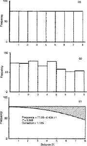
Fig. 7.2.  A schematic diagram for the basic idea behind line transect sampling.  You don't need to be able to read the numbers, just try to grasp the central concept.  The X-axis shows eight distance categories (all objects detected in the first x meter interval, all objects in the second x meter interval, etc., where x will be determined by the species being estimated and the nature of the habitat).   The Y-axis shows the percentage of the total detections represented in each of the given distance intervals.
TOP PANEL.  If a population were uniformly dispersed and we conducted a complete census we should come up with a histogram of objects at intervals from the center line as shown in the top histogram.  That is, we would fully detect all objects, regardless of distance from center line — so all the bars in the histogram would be of equal height,
MIDDLE PANEL.  In practice, however, detection will decrease with increasing distance from the center line, as shown in the middle histogram.  These bars are just one particular example of the general kind of pattern we should expect from actual field data — we should see a 'shoulder' of large bars near the center line, and then the bars furthest from the center line should be noticeably smaller.
BOTTOM PANEL.  The challenge is to estimate the 'undetected' objects shown by the shading in the bottom diagram.  The method of line transect sampling does just that and allows us to compute an estimate of the total population (shaded plus unshaded portions of the bottom diagram corresponding to the 'full' histogram at the top).  One more point: the actual estimator in line transect sampling is called f-hat(0) -- where the zero in brackets refers to the objects detected at zero distance from the line.  Think about why that first bar should be a good basis for going from the middle panel (actual field detections) to the top panel (hypothetical perfect knowledge).

Real-world issues:

Animals move
Animal response behavior and our ability to detect them may change during the survey
           (because of changing wind levels and other factors.)
Individual animals may respond differently.

Here are the three criteria that Burnham and Anderson (1980) set for a good model of f(x) -- f (x) estimates how much of the total probability of detecting an object occurs at distance x from the transect line.  [As shown in both the middle and bottom panels, f (x) will decline as x increases].
        1) General robustness (flexible enough to fit a range of actual shapes of detection probability -- that is, the range of shapes that might occur for the shaded 'undetected' part of the upper right in the bottom panel of Fig. 7.1).
       2) Robust to pooling (variation in detection probability factors - some unknown)
       3)  Shoulder near zero -- near the centerline we expect to see almost all the animals (the 'shoulder' but then the detection probability drops off from some moderate distance.
      4) Efficient estimator (low variance, low bias)

Layout/design considerations: We could use any of a series of different possible layouts. These could include connected lines with 'kinks' that change angle, systematic designs that cover the study area in a regular design, or subdivided plots that partition the study area.
Somehow, though, we should try hard to incorporate some randomization. This could involve a randomly selected starting point on the perimeter, a randomly chosen angle for the parallel transect lines, or some other way of avoiding systematic bias (again, at all costs we want to avoid some obvious source of bias such as paralleling ridge tops.

SUMMARY of considerations in designing the layout:

Define the population of interest
Delimit the population (figure out the logical and logistically feasible boundaries)
Devise a sampling scheme that truly samples the population of interest
Conduct a survey the gathers the required data
Goal of the design: Sample the population of interest in a way that yields an adequate representation of reality

To meet the goal in practice:

Every member of the population must have an equal probability of being sampled
           (can't have submerged whales that are not susceptible to sighting)

Must have adequate replication (adequate sample size)

Sample must have adequate spatial dispersion (and possibly temporal dispersion)

Must avoid correlation between transect orientation and particular features of the landscape (such as ridges or valleys). It's acceptable to have one line (of many) that (by chance) aligns with the environmental feature (road, river), just not that they ALL do so -- that may produce bias.

Must bring randomization into the design process at some point -- the more the better, but if nothing else then a random starting point or random direction (for parallel or systematic designs).

Data that must be collected for line transect sampling:

Total length of lines traversed, L (most applications will include replicate lines; these may be parallel to each other, zigzag in random directions or apply a form of stratified randomization)

Number of objects detected, n.

Number of individuals within each object (e.g., birds per covey)

Perpendicular distance, x_i from transect line to object i (i = 1 to n). It is usually best also to measure angle and distance from detection point to object (since many objects will be detected before they are directly perpendicular to the transect line).
Maximum distance of detection will be w*(the one-way width of the transect detection area). Total 'detection' area will then be 2Lw*.

Sample size (n) of number of objects detected should be no less than 40.

Go to optional web page with greater detail on Line Transect estimation (and Mark-Recapture)

References on population estimation:

Burnham,K.P., D.R. Anderson, and J. L. Laake. 1980. Estimation of density from line transect sampling of biological populations. Wildlife Monographs No. 72.

Caughley, G. 1977. Analysis of Vertebrate Populations. Wiley, New York.

Eberhardt, L.L., and M.A. Simmons. 1987. Calibrating population indices by double sampling. J. Wildl. Man. 51: 665-675.

Jolly, G.M. 1965. Explicit estimates from capture-recapture data with both death and immigration -- stochastic model. Biometrika 52: 225-247.

Kalka, M.B., A.R. Smith, and E.K.V. Kalko. 2008. Bats limit arthropods and herbivory in a tropical forest. Science 320: 71.

Krebs, C.J. 1989. Ecological Methodology. Harper & Row, NY.

Rotella, J.J. and J.T. Ratti. Test of a critical density index assumption: a case study with gray partridge. J. Wildlife Manage. 50: 532-539.

Schnabel, Z.E. 1938. The estimation of total fish in a lake. Am. Math. Mon. 348-352.

Schumacher, F.X., and R.W. Eschmeyer. 1943. The estimation of fish populations in lakes and ponds. J. Tenn. Acad. Sci. 18: 228-249.

Seber, G.A.F. 1965. A note on the multiple capture-recapture census. Biometrika 52: 249-259.

Woolfenden, G.E. and J.W. Fitzpatrick. 1984. The Florida Scrub Jay: Demography of a Cooperative-breeding Bird. Monogr. Pop. Biol. 20. Princeton Univ. Press, Princeton, N.J.

Some web-based resources for analysis of populations:

http://www.stanford.edu/group/CCB/Eco/popest2.htm Stanford U. population estimation page

http://canuck.dnr.cornell.edu/misc/cmr/
            Evan Cooch (Cornell) page of mark-recapture software and sources

http://www.cnr.colostate.edu/~gwhite/mark/mark.htm
            Gary White (CSU) page of software etc.

Web site for the current documentation on line transect sampling using the program DISTANCE
           http://www.colostate.edu/depts/coopunit/distancebook/download.html
           Burnham and Anderson Distance manual for software (including line transect analysis) in pdf format

End of web-only material.

Return to top of page                Go forward to notes for Lecture 8,  1-Feb