Lecture notes for ZOO 4400/5400 Population Ecology
Lecture 8, (Friday, 1-Feb-13)
What is demography, and why does it matter?
Type I-III survivorship curves, patterns of mortality, Simpson's paradox.
Required reading: Gotelli text, pp. 50-56 (in "Required Readings>Feb" folder on WyoWeb)
Suggested reading: Keyfitz: heterogeneity and selection, Simpson's paradox (in "Suggested Readings>Feb" folder on WyoWeb)
Return to Main Index page
Go back to notes for Lecture 7, 30-Jan
Go forward to notes for Lecture 9, 4-Feb
Excel spreadsheet for Type I, II, III survivorship curves is in WyoWeb handouts folder.
Demography: what is it?
I will now turn to the compilation and analysis of demographic data -- demography is the analysis of vital rates (population statistics such as birth rates and death rates). The roots of mathematical demography lie in problems related to urban human populations -- insurance, taxation calculations, the study of disease epidemics. One interesting problem here is that processes that occur at the level of the individual (you either live or die, 0 or 1) have emergent properties at the level of populations (the probability of dying, for a five-year-old bull elk, is 0.227 +- 0.83 [meaning that, on average 22.7% of these bulls die, with a standard deviation around that average of plus or minus 8.3%]. I will list several reasons for knowing something about demography, and then turn to analysis of broad patterns of mortality, including the problem of senescence. In this course we will approach demography largely from the angle of matrix projection models. Before introducing matrix models, I will discuss broad patterns of mortality and natality in natural populations.We will look at patterns of mortality and natality, put those together into life tables, and then see how we can use the data in matrix projection models.
Why does demography matter when studying natural populations of animals or plants?
1. Extinction is a demographic process (deaths outweigh births)
2. Allows us to move from simple, disorganized counting to
a) understanding or predicting process and pattern
b) having a firm statistical basis for comparison and decisions [power of the test & accepting null when false: Taylor& Gerrodette, 1993 pointed out that Russ Lande's (1988a) assessment of l = 0.96 for Spotted Owls, Strix occidentalis, had low power and therefore could not be said to differ from 1.0]
3. Some definitions and contrasts
a) projection vs. forecasting. Projection says what would happen if current conditions hold (like the speedometer of car vs. forecasting, which tries to predict what will happen).
b) Ireland vs. Iceland (when not how many). Irish family sizes are more than twice those of Iceland, yet Iceland has a higher growth rate. Why? Because people in Ireland start their families much later. Timing of reproduction as well as quantity makes a huge difference to population dynamics in age-structured populations.
4
.
Demography vs. genetics (
Lande,
1988b) [but see
Lynch, 1996 for why
quantitative
genetics might really matter] :
a) populations collapse first
(for
demographic reasons) then
face inbreeding (genetic) problems.
b) genetic 'treatments' can be
applied
only to a
few showcase, charismatic species.
c)
appropriate uses of genetics: not
to determine
health, but as a tool in surveying
diversity, in decision-making about distinctiveness of taxa,
and as a way of making demographic
inferences.
Is this endangered taxon distinct enough to merit protection (Dusky Seaside Sparrow case)
5. Other approaches to population
dynamics (besides
the matrix-based projection models that will be our primary emphasis)
Patterns of
mortality
Any demographic analysis will almost
certainly incorporate
the two fundamental forces of birth and death. What are the
patterns
of birth and death in natural populations?
We will start on the topic of survival and mortality by discussing Type I, II and III survivorship curves.
Fig. 8.1. Type I (green), II (blue) and III
(red) survivorship. The Y-axis is survival measured as the logarithm of
lx, where lx is the proportion of individuals surviving to
age x, the Type I is characteristic
of humans, elephants and other long-lived organisms with low infant mortality.
Type II is characteristic of birds and other organisms with
relatively constant mortality rates throughout the lifespan. Type III
is characteristic of organisms with very high juvenile mortality
such as oysters, insects, some plants. The few individuals that become
established may then have high survival rates. Note that the plot is
semi-logarithmic -- that is, the Y-axis is the natural logarithm of the lx
values. MANY species will have curves that do not follow any of the three
types. They may start with low survival, then have a phase of fairly constant
mortality, followed by rapid senescence later in life -- a mix of all three
curves. The reason for presenting these curves is to provide a framework
for thinking about broad patterns.
Note that the
logarithmic
scale means that we have exponential decay for the blue
straight
line. This is the same idea as that presented in Lecture 5, where
the log of N is linear against time for exponential growth, and
a more complex log term is also linear for logistic growth. We could, therefore, calculate a constant "halving" time, by analogy with doubling time under exponential growth. An
early
discussion of these curves was by Deevey (1947).
We will discuss lxmx
schedules in Lecture
9. See Gotelli text, pp. 50-56 for further details (he calls
fecundity bx, rather than mx).
Excel spreadsheet for Type I, II, III survivorship curves is in WyoWeb handouts folder. The spreadsheet shows how values were calculated from an lxmx schedule, as well as how the plot would look if the values were not
log-transformed.
Who dies?
Mortality is rarely random. That is, it almost always has greater impact on certain classes of individuals than
others. Examples include high mortality of newborns and elderly compared to
prime of life, higher predation on incubating females, higher mortality of displaying
male frogs or elk, differential harvest and many other potential factors.
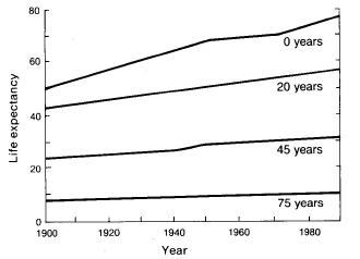
Fig. 8.2 A human example of differential mortality/survival.
Modern medicine and public health programs (e.g., better waste treatment)
have had a tremendous effect on life expectancy -- most dramatically for
infants. The rise in life expectancy since 1900 is negatively correlated with age.
I will give two examples of patterns of mortality. The first shows differential mortality as a function of social status
(roughly equivalent with age) in cooperative-breeding Florida Scrub-Jays.
Unequal mortality as a function of age or social status
A 1979 epidemic in Florida Scrub-Jays dropped total jays per 40 ha from 13 to 7.5 (a loss of 6.5 jays per 40 ha), but only
2 of the "6.5 lost" were breeders (breeder density went from 8 per 40 ha to 6 per 40 ha). Thus the mortality had
relatively less effect on the breeding population than on the "surplus" individuals. This nonrandom
mortality will tend to stabilize the population dynamics because the core breeding population varies much less than fringe of older and younger
individuals. (Woolfenden and Fitzpatrick, 1984).
Patterns of mortality across different taxa: What types of animals are generally very long-lived for their body size?
Birds compared to mammals.
Fig. 8.3. Longevity of birds (upper line) vs. that of mammals (lower line) as a function of body mass.
For their size, birds live considerably longer than mammals. Notice that this is a log-log plot, so what look like smallish
differences are sometimes many times different. (From Austad and Fischer, 1991)
Why that might be? Now let's add two
long-lived taxa
to that. First, bats.
Fig. 8.4. Maximum longevity of species of bats (squares, all but one of which of which are above the line)
compared to the regression line for nonflying eutherian (placental) mammals. Being above the line means that a species lives a
long time for its body size. Note that both homeothermic (open symbols) and heterothermic (filled symbols)
bats have longevities above the line. That suggests that whether or not
bats "save their batteries" by hibernating/going into torpor is not the
primary determinant of their longevity. (Circles are marsupials).
(From Austad and Fischer, 1991)
What else? Tortoises. Hmm. What do birds and bats have in common? Can we make that general enough to encompass tortoises?
One hypothesis is that longevity is related to metabolic rates. The two graphs given below show why that is unlikely.
Fig. 8.5. Metabolic rates of birds and mammals as a function of body mass.
Note that nonpasserine birds have metabolic rates essentially equivalent to those of mammals.
If the metabolic rate hypothesis were a good explanation for longevity we would expect
that only passerine birds would differ from mammals in longevity. (From Austad and Fischer, 1991)
Given the comparative metabolic rate data above, what are the observed patterns of longevity? Do they fit the metabolic rate
hypothesis?
Fig. 8.6. Longevity of birds and mammals as a function of body mass. The pattern is inconsistent with the
prediction of the metabolic rate hypothesis. (From Austad and Fischer, 1991)
What could explain the observed patterns? The invulnerability to predation
hypothesis.
Derek Pomeroy
(1990) and
Austad
and Fischer (1991) developed a hypothesis for longevity based on
vulnerability
to predation (or any other extrinsic force of mortality; predation is
likely
to be one of the most important forces for natural populations). Flight
makes birds and bats able to escape quickly PLUS they have 3
dimensions in which to flee instead of two. Austad demonstrated
extended
longevity experimentally by introducing opossums to a predator-free
island in Georgia. Life expectancy almost doubled. Interestingly, some
physiological
responses also occurred, such as decrease in collagen cross-linking.
The
experimental results suggest that lifespan itself is subject to (fairly
rapid) evolutionary change. Back to the tortoises. Their shells
confer
an important protection against predation.
Yet another example: ground-displaying
lek-mating birds
such as Sage Grouse and Black Grouse (4-7 year) have far shorter
lifespans
than do aerial displaying lek-mating birds such as manakins (10-20
years).
This difference in lifespan is the reverse of what we'd expect from
body
size -- the grouse are 177 times heavier than the manakins.
Flight
confers protection from predation in at least two major ways -- faster
zero-to-top-speed acceleration, three-dimensional escape volume rather
than two-dimensional surface.
Nevertheless, everything dies eventually.
Why?
Two major hypotheses exist to explain the phenomenon of senescence (Williams,
1957):
I. Pleiotropy (tradeoffs).
Pleiotropy
refers to multiple effects from a single gene or trait. In this context
it means that a gene that has beneficial effects early in life will be
selected for, even if it has detrimental effects later in life.
II. Lack of selection
against mutations
with late effects. If a mutation arises that has effects
late
in life selection barely "sees" it, because most of the reproductive
span
is already over and the fitness cost is low (compared to a mutation
with
an onset at the peak of the reproductive value curve).
Both of the above hypotheses depend on the decline
of reproductive value with age. Why does senescence occur?
Thought experiment.
Imagine that we have organisms with a potentially infinite life span.
In
practice, even in the absence of any intrinsic decline in health or
vigor
with age, accidents and disasters would make the life span finite. As
soon
as "accidents" happen that change the lifespan from theoretically
infinite
to actually finite, we will see a reproductive value curve that
declines
to zero at the end of the life span. As soon as the reproductive value
curve declines with age, selection will favor one of the two mechanisms
listed above (or both).
[A
considerable
body of theory applies to this problem of "accidental" death. Much of
it
was developed for estimating industrial/commercial problems such as the "lifespan" of light bulbs. Much of that theory of breakage and
attrition
applies to evolutionary demography. The contributions work both ways --
economists and engineers have learned a great deal from evolutionary
demographers, and likewise biologists have learned useful mathematical and modeling
techniques from economic and industrial models and techniques].
Nevertheless, senescence in birds at least, has been
difficult to detect. Why? Senescence and heterogeneity. Let's start
with an example of something called Simpson's paradox:
We examine family sizes of French speaking (generally Catholic) Canadians and English-speaking (generally Protestant)
Canadians. For Canada as a whole the numbers are:
French speaking English speaking
Canada
1.85
1.95
Now let's break Canada into two compartments
-- the
two compartments together account for all of Canada. The statistics are:
Quebec
1.80 1.64
Other provinces
2.14 1.97
So, in Canada as whole the French speakers
have a smaller
family size, and yet in each of the two compartments that make up the
whole,
they have a LARGER family size. How can this be???? How can each of the parts have a pattern that is different from that of the whole?? The explanation is called Simpson's paradox.
References:
Austad,
S.N., and K.E. Fischer. 1991. Mammalian aging, metabolism, and ecology:
evidence from the bats and marsupials. J. Geront. 46: B47-53.
Deevey,
E.S., Jr. 1947. Life tables for natural populations of animals. Quart.
Rev. Biol. 22: 283-314.
Hanski,
I. 1998. Metapopulation dynamics. Nature 396: 41-49.
Hastings,
A. 1994. Metapopulation dynamics and genetics. Annual Review of
Ecology
and Systematics 25: 167-188.
Holmes,
D.J., and S.N. Austad. 1994. Fly now, die later: life-history
correlates
of gliding and flying in mammals. J. Mammal. 75: 224-226.
Judson,
O. P. 1994. The rise of the individual-based model in ecology. TREE 9:
9-14.
Kareiva,
P., and U. Wennergren. 1995. Connecting landscape patterns to ecosystem
and population processes. Nature 373: 299-302.
Keyfitz,
N.
1985. Applied Mathematical Demography. Springer-Verlag, NY.
Lande,
R. 1988. Genetics and demography in biological conservation. Science
241:
1455-1460.
Lande, R. 1988. Demographic models of the northern spotted owl (Strix occidentalis caurina). Oecologia 75: 601-607.
Lindenmayer,
D.B., and R.C. Lacy. 1995. Metapopulation viability of leadbeater
possum, Gymnobelideus
leadbeateri, in fragmented old-growth forests. Ecol. Applic. 5:
164-182.
Liu,
J.G., J.B. Dunning, and H.R. Pulliam. 1995. Potential effects of a
forest
management plan on Bachman's sparrows (Aimophila aestivalis):
linking
a spatially explicit model with GIS. Conserv. Biol. 9: 62-75.
Lynch,
M. 1996. A quantitative-genetic perspective on conservation issues. pp.
471-501 In Conservation Genetics: Case Histories from Nature
(J.C. Avise and J.L. Hamrick, eds.). Chapman & Hall, NY.
Morris, W.F., and D.F. Doak. 2002. Quantitative Conservation Biology.
Sinauer Associates, Sunderland MA.
Pomeroy, D. 1990. Why fly? The possible benefits for lower mortality. Biol. J.
Linn. Soc. 40: 53-65.
Rose, M.R. 1991. Evolutionary Biology of Aging. Oxford Univ. Press, Oxford.
Simberloff,
D. 1995. Habitat fragmentation and population extinction of birds. Ibis 137: S105-S111.
Taylor, B.L., and T. Gerrodette. 1993. The uses of statistical power in conservation biology: the vaquita and northern spotted owl.
Conserv. Biol. 7: 489-500.
Williams,
G.C. 1957. Pleiotropy, natural selection and the evolution of senescence. Evolution 11: 398-411.
Woolfenden, G.E. and J.W. Fitzpatrick. 1984. The Florida Scrub Jay: Demography of a
Cooperative-breeding Bird. Monogr. Pop. Biol. 20. Princeton Univ. Press, Princeton, N.J.
§§§§§§§§§§§§§§§§§§§§§§§§§§§§§§§§§§§§§§§§§§§§§§§§§§§§§§§§§§§§§§§
Return to top of page
Go forward to notes for Lecture 9, 4-Feb