Lecture notes for ZOO 4400/5400 Population Ecology
Lecture 13 (13-Feb-13) Some thoughts on working with equations and graphs.
Return to Main Index page
Go back to notes for Lecture 12 ,
11-Feb
Go forward to Lecture 14, 18-Feb-13
Today's lecture (different in-class version may be presented by TA Sara Decker) will be a sidetrack that provides you with some useful tools both for the this course and for any
future coursework or professional work you do that has quantitative implications.
Let's start with graphs, since we have been working extensively with them in the recent course topics.
I. Axes labels. If you are building a graph, make sure to label your axes and (almost always) to put a
scale on them. Remember that (usually) the X-axis (abscissa, horizontal) is for the predictor
variable (the causative factor, the measurement domain [such as time]) whereas the Y-axis (ordinate, vertical) is
for the response variable (the dependent variable, the result we're interested in).
In a few cases (such as the 1-dimensional maps for the discrete logistic or the phase plane plots for the Lotka-Volterra equations), the axes
won't fit the "usual" X/Y, independent/dependent mold. In that case, think about what they do represent.
II. Extreme thinking. It often really pays to think of the maximum or minimum values that are reasonable. On one
exam, some students ran into trouble with one of the plots because they changed values in such small increments that they couldn't see the
"curve". Yes, the Laramie plains are flat, but at a larger scale they are part of the curved sphere that forms the surface of Earth.
At a very small scale, they have lots of small hills and valleys (that affect snow accumulation, provide refuge for small mammals, etc.). What is the smallest feasible value? What is the largest feasible value? What happens if we set a variable to zero?
Example: When thinking of the logistic equation, two useful extremes are N = 0 (leads to dN/dt = 0) and N = K (again leads to dN/dt = 0). Go even further to N = 2K. In that case, dN/dt is strongly negative. As we now know, dN/dt goes to its maximum midway between 0 and K.
Plotting lines on graphs using extremes: In many cases, when you want to plot an equation (linear or non-linear) the easiest way
is to look for any "easy" or "extreme" solutions. If you have two variables (X and Y,
or N1 and N2), it is often easiest to set one of the variables to zero and then solve for the other variable. Setting one
variable (say X) to zero, means that your solution will be a point along an axis. That point will be {0, Y-solution} or
{X-solution, 0}. For the competition isoclines, the nice thing was that you could
get both ends of the line this way. Find a point on the Y-axis (the Y-intercept or the b of the equation Y = b - mX), find a point on the X-axis, connect the dots with a straight line, and you have the isocline.
III. Fixed system-governing lines vs. particular-case trajectories. Homework 5 is a good illustration of the difference
between general (system-wide) aspects of graphical analysis and particular cases that obey the rules of that system. When we solve for the
isoclines, we produce lines of the form Y=b - mX, where b is the Y-intercept, and m is the slope (preceded by a negative
sign in the competition case). These lines create "forces" that drive particular cases, wherever those particular cases happen to
be. That is, the "starter values" I gave you are particular examples of one out of many possible particular states: we might, for example,
start with 200 white-tailed deer and 350 mule deer. On our graph, that particular case is a point {N1, N2} which we can also
consider to be an X/Y coordinate {X, Y}. Any point on the graph {restricted to N1 >= 0, N2 >= 0} is a
possible particular case. The forces that work on those points, and that cause
them to follow trajectories toward a destination are equations described by lines. This anywhere-is-ok ability is why such plots are called phase plots. In other cases (e.g., the plot of dN/dt against N) the only meaningful places are along the curve. Randomly picking some other X-Y coordinate just makes no sense.
Let's take a very different example and think about what the plot means -- the solution of the
differential equation for logistic growth (the familiar sigmoid curve of population growth). Is that a fixed, system-governing curve or a
particular-case trajectory? Despite the fact that you almost always see the "logistic" visually depicted that way, the familiar
sigmoid is just one (of many) particular realizations of a "rule" of attraction, toward the carrying capacity, K.
The books almost always show the trajectory for a population that starts with a very few animals (low, but not at zero,
on the Y-axis, with the Y-axis depicting N, the population size). But what if we started with a population
greater than K? Just less than K? Above K/2 but < K? All of these particular starting points move along a trajectory
(and from above K/2, it's not even sigmoid!) toward K. The (usually invisible/not depicted)
force-line is an isocline! That isocline (along which the population size has no intrinsic tendency to increase or decrease) is a horizontal
line from N=K at t = 0, to N=K (still) at t = tmax.
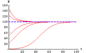
Fig. 25.1. Logistic growth from several different starting points, moving toward the system-attractor (isocline).
Each red line is a particular realization of the solution of the differential equation (using a particular starter N0 value).
The dashed blue line is the isocline, representing the solution from setting dN/dt to zero (the solution is the very simple
expression N=K). Because the N=K isocline is an essentially global stable equilibrium (what values don't
converge to K?) many different starting points move toward the isocline. Carrying capacity (K) is 100.
Question to ponder: What would a a graph equivalent to Fig. 25.1 look like for the sigmoid
harvest function of Fig. 23.6? That is, if we plotted multiple starting points (say, in red) and "isoclines" (say in blue dashes), how
would the resulting graph resemble and differ from Fig. 25.1?
IV. When is an equation linear vs. non-linear? Just the fact that an equation has squared or exponential terms in it, does
not make it non-linear. Squaring, exponentiating or taking the natural logarithm of a constant does not change the linearity of an
equation. The non-linearization has to be acting on a variable.
 Eqn 25.1
Let's graph this equation:
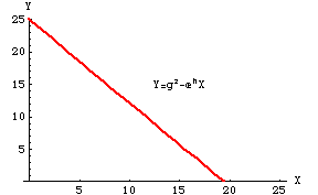
Fig. 25.2. Graph of Eqn 25.1. Despite the squared and exponential terms, the graph is linear. That is because Y is
linear with respect to X. The squaring and exponentiating is all acting on constants, which simply changes their value -- it does
not affect the relationship between X and Y.
V. Setting something to zero -- difference between stability analysis and "getting rid" of a variable. Just because you are
setting things to zero (using a similar numerical trick) doesn't mean you are doing a completely parallel analysis.
In some of the paired logistic competition analyses that involved isocline work, some of you seemed to be confused
about what you should set to zero, and what it meant when you did. The zero-settings occurred at two different stages in the analysis and
had very different reasoning behind them.
First zero-setting: we set dN/dt to zero to do a stability analysis (i.e., to get an isocline). That gives us a solution (in symbolic form) that includes two variables (N1 and N2) and some constants (K's, gammas). Here the purpose is to get a general solution for equilibrium.
Second zero-setting(s): Hmm... we have one equation, in two unknowns -- this is not a good thing
in the world of algebra. Solution? First, we set N1 to zero (useful because it gives us a toehold on one of the axes).
That gives us Point Number One (at zero on the N1 axis and up along the N2 axis). Then set N2 to zero. That gives us Point Number Two (at zero on the N2 axis and out
along the N1 axis). Then we can connect those dots to get the straight-line isoclines. Here the
purpose is to calculate two particular equilibrium values (where the isoclines hit the axes).
Case history: Why solve two different equations for the same variable (N2)?
Say, for example, we are solving the N1 isocline for a stable coexistence case (by setting dN1/dt to
zero) using the first kind of zero-setting to get:
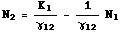 Eqn 25.2
Why did I set it up that way and solve the N1 isocline in terms of N2? Because that form of the
(still completely symbolic) solution in Eqn 25.2 is arranged to be in the form:
 Eqn 25.3
where b is the Y-intercept, and m is the slope. Here, the slope is one over the gamma12 term and the
Y-intercept is the "visitor's" K divided by the gamma that describes the impact of N2 on N1.
Putting N2 on the left hand side makes it easy to do the second kind of zero-setting and solve the linear isoclines for the
places where they will hit the two axes. Let's review what that zero-setting involves.
Second kind of zero-setting, part 1: we set N1 to zero and get b (the Y-intercept) as
K/gamma12. Now.... because we set up the Eqn 25.2 in the special form of 25.3 we don't
really need to do the second zero-setting, because we could "see" the Y-intercept in our equation (but it can't hurt to do it
anyway, as a check).
Second kind of zero-setting, part 2: we set N2
to zero and get the X-intercept, which is simply K1 (do the algebra on Eqn 25.2 and assure yourself of this).
So, in the first case, we were getting a general solution/isocline/system
attractor equation for stability analysis. In the second and third cases, we were setting each of the variables to zero for the purpose
of getting particular (extreme) points for plotting endpoints of those isoclines.
Because we do not see any squared or exponential or logarithmic terms in the equations, we can be sure that the equation is linear. We
can, therefore, simply connect the dots to get the isoclines. All of this is working with the general system-attractor isocline system
(not particular cases) but the first zero-setting helps uncover the general equation and the other zero-settings give us useful particular end
points (i.e., where the isoclines hit the axes).
§§§§
§§§§§§§§§§§
§§§§§§§§§§§§§
§§§§§§§§§§§§§§
§§§§§§§§§§§§§
§§§§§§§§
Return to top of page
Go forward to Lecture 14 , 18-Feb-13