Lecture 14 (Monday, 18-Feb-13)

Matrix models (cont.). Approach to equilibrium.

Return to Main Index page      Go back to notes for Lecture 13,  13-Feb   Go forward to notes for Lecture 15,  20-Feb

Go to notes on matrix algebra (e.g., how to multiply matrices)

Download Excel spreadsheet for projecting a census vector

(Software that calculates the eigenvalues and eigenvectors is now available as an Excel add-in at http://www.cse.csiro.au/poptools/)

       (I use the programming language/mathematical software Mathematica)

Population's approach to equilibrium (stable age distribution).

Now let's try a variant of a matrix/life cycle graph but with real (preliminary) data for endangered black-footed ferrets.

Reproduction starts at the end of the first year. The main change from the matrix and life cycle graph at the end of Lecture 12 is, therefore, that our starter matrix now has a "self-loop" in the upper left hand corner (an arc that points back to the node it came from).

Remember that the F_i fertility terms include a survival term, P_i, for the mothers. We counted mothers just after a breeding pulse (post-breeding census).  In order for the mothers to reproduce at the end of our one-year census interval, they must survive through the interval (with probability P_i).

Figure 14.1 (compare to Fig. 12.1) shows the change we are introducing, which involves the self-loop on Node 1:

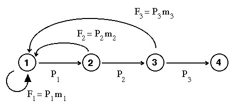
Fig. 14.1. Life cycle graph of black-footed ferrets, for showing approach to stable age distribution (SSD) and other matrix phenomena.
The difference between this graph and that of Fig. 12.1 is the addition of a self-loop for reproduction
at the end of the first year (production of more beginning-of-first-year animals by end-of-first-year animals).

Question to ponder:  Since we know that P₃ = 0.346, what is m₃?

Crunch the revised matrix: 

0.691	0.898	0.606
0.464
	0.534
		0.346

Fig. 14.2.  Projection matrix for black-footed ferrets used for the 'age wave'
    demonstration.  The matrix has the same number of rows (4) and columns (4)
as the life cycle graph (Fig. 14.1) has nodes (4).  The fertilities (F_i) are in the top row,
while the annual survival rates (P_i) are in the subdiagonal.  Each cell in the matrix
corresponds to an arc in the life cycle graph.  Where no arrow occurs, the corresponding
matrix cell is empty or zero.

and we get: l = 1.16

The reproductive value (RV) vector is:  {1, 1.01, 0.52, 0}

The stable age distribution (SSD) is:

0.61  (i.e., at the time of the census, 61% of the population are 1st-year individuals)
0.24
0.11
0.03

The scalar product (SP) is 0.91 (given the RV, SSD and SP you can calculate the sensitivities yourself, using Eqn 12.1)

Now, let's say we start with a census vector that is NOT at the stable age distribution (i.e., it is not at equilibrium) and project it for 10 years. Say, for example that we start with 25% of the population in each of the 4 age classes at time t = 0 (second bar in Fig. 13.3). Here's what happens to the proportions :

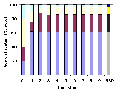
Fig. 14.3. Age distribution for the black-footed population with four age classes projected over nine time intervals. At time t = 0, the four age classes account for the given proportions of the population (20% 1st-year, 20% 2nd-year, 40% third-year, and 20% 4th-year; each of the colors is the proportion in the age-class). By t = 9, the population has essentially converged on the stable (st)age distribution (SSD) shown at the far right in darker colors. Notice that the over-representation of certain age classes (e.g., the third-year class shown in white) is 'squeezed out' in a wave-like pattern. SSD values from bottom to top in stacked bar at right: Gray (bottom): equilibrium percentage of 1st-year individuals; black: equilibrium percentage of 2nd-year individuals; yellow: equilibrium percentage of 3rd-year individuals; dark blue (top): equilibrium percentage of 4th-year individuals. Observed values (t = 0 to 9): Light blue: observed proportion of 1st-year individuals; purple: observed proportion of 2nd-year individuals; white: observed proportion of 3rd-year individuals; light green: observed proportion of 4th-year individuals. The proportions were calculated by sequentially right-multiplying an initial census vector (e.g., 20, 40, 20, 20) against the Leslie matrix shown  in Fig. 14.2.

Let's try the same thing but starting with all the individuals in the 3rd age-class.

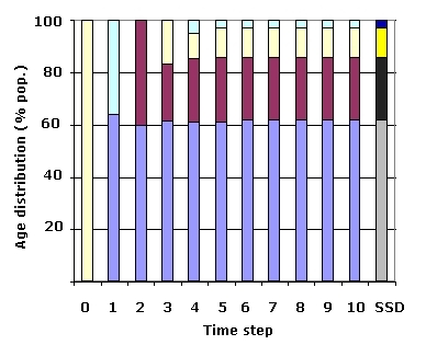
Fig. 14.4. Approach to the stable age distribution by a population that starts at t=0 with
all 100 individuals in the third age-class.  Notice the dramatic fluctuations on the way to time step 4. 
Compared to the projection series in Fig. 14.3. the proportions here approach the SSD values slightly
more slowly and are slightly further from the SSD at t = 10.
All bars have the same meanings as in Fig. 14.3.

The "waves" in the age structure disappear as we approach equilibrium at the stable (st)age distribution, SSD. Note that the equilibrium for the matrix model is defined in terms of the age structure. That contrasts with the stable equilibrium in the logistic model, which was defined in terms of population size (N = K).

Questions to ponder.
        If I started with 0 1^st-, 2^nd-, and 3^rd-year individuals and 100 4^th-year individuals and projected to the next census interval, how many would I expect to have at the next census?
Alternative question. What is the reproductive value (value as a seed for future population growth) of a 4^th-year individual?
         Does that help answer the first question?
If a life cycle graph has five nodes, how many possible arcs does it have?  Is a life cycle likely actually to have that many arcs (indeed, can it, if it is an age-classified model)?

Here's the matrix of sensitivity values (remember, each number corresponds to an arc in the life cycle graph)

0.67	0.27	0.12
0.68
	0.14
		0

Fig. 14.5.  Matrix of sensitivity values for the black-footed ferret values.  l is most sensitive to a change in first-year survival.  First-year survival is s₂₁ = 0.68, corresponding to the P₁ arc. l is not at all sensitive to a change in third-year survival. 

The highest-sensitivity arc comes from the node with the highest SSD (0.61) and goes to the node with the highest RV (1.01).  Again, "size of source (SSD) times reproductive value of target (RV)" tells us about the sensitivity. 

The matrix of elasticities is:

0.4	0.21	0.06
0.27
	0.06
		0

Fig. 14.6. Matrix, E, of elasticity values, with cells e_ij, for the black-footed ferret model.  Note that the arc to which l is most elastic is F₁.  That's because the elasticities (impact on l of a proportional change in a vital rate) are computed as the sensitivities weighted by the value of the original arcs.   Because F₁>> P₁, it follows that e₁₁ > e₂₁. 

Overview of matrix-based analyses:

Purpose:

Analysis of complex age- or stage-structured populations
                    (vs. 'simpler' dynamics of populations with non-overlapping generations).

Analysis of which life cycle transitions (e.g., adult survival, growth probability for yearling trout, offspring production by yearlings) have a large impact on population dynamics.

Measures produced:

Sensitivity: effect on lambda of a small absolute change in a given vital rate
Mathematically, the sensitivity is the product of the stable (st)age distribution value of the node from which the arc originates, times the reproductive value of the node to which it points (that is it weighs the reproductive value of the destination, by how much flows into it along that arc). I suggest memorizing this verbal definition.

The sensitivities reflect
        how valuable the destination node is (RV)
               times
        how large the source node is (SSD).
(Value of target) times (size of source)

             [See Caswell, 20019, p. 208, if you wish to pursue this].

Elasticity: effect on lambda (l) of a small proportional change in a given vital rate.  Calculated by weighting the sensitivities by the value of the original arc/matrix cell.

Population growth rate (l, the dominant eigenvalue)

Stable (st)age distribution (SSD, right eigenvector)

Reproductive values (RV, left eigenvector): reproductive value curves tend to peak at age of first reproduction (unless survival or fertility prospects continue to increase dramatically)
        Reproductive value is the value of an individual of a given stage as a
                      seed for future population growth (in first stage equivalents).   
        Reproductive value represents an individual's current and expected future offspring production,
                       weighted by its survival prospects.
            That is, the reproductive value weighs all the pathways along which we can move from a given node
                       back to the first node (new recruits).
            Post-reproductive individuals have a reproductive value of zero

Generation time

Average age of a stage (for life cycles analyzed by size, social status or some other way that differs from classic age-classified Leslie matrix).

Guidance for field effort and management:

•  Which vital rates require the most careful measurements (the most sensitive)

•  If we want to manage population dynamics where could we make changes that would have the largest impact?

•  Example: let's say we find that cowbirds are a major contributor to the decline of a passerine bird.
By doing a sensitivity analysis of the life cycle of the cowbirds we could find out where to put our efforts into cowbird control.

Assumptions:

Vital rates do not change over time (no effect of environmental stochasticity)

Evenly spaced census intervals at a particular time in the cycle (usually an annual post-breeding census for most vertebrates)

Birth-pulse reproduction(as opposed to birth-flow)

We have measured the vital rates reasonably accurately
(Accuracy of measurement of sensitive transitions is the most critical)

We have accounted for all possible transitions in the life cycle

No density-dependence

{We can add stochasticity or density-dependence to matrix models, we just haven't done that here}

For reproductive values and stable age distribution, sensitivities and elasticities, we are also assuming the population is at equilibrium.  That is, the population has gone through any transient dynamics caused by not starting at the stable age distribution. 
         {Look back at the changes in the age structure in Figs. 13.3 and 13.4 for examples of how the transient dynamics gradually smooth out and the population reaches equilibrium -- in a matrix model equilibrium means the population has achieved the stable age or stage distribution}.

Things the analysis won't do for us: Even if we know which are the most sensitive transitions, we may not be able to do anything about them. For example a manager who deals with a migratory population only on the breeding grounds may not be able to affect overwinter survival even if that is the most sensitive transition. (Nevertheless, it may be important that she or he know what is most important).

§§§§§§§§§§§§§§§§§§§§§§§§§§§§§§§§§§§§§§§§§§§§§§§§§§§§§§§§§§§§§§§§§§§§§§§§§§§§§§ß

The material below is not anything I will test directly, but studying it, at least to the point where it makes sense (even if you couldn't do it on your own) is likely to help make the matrix models more comprehensible. 

Some notes on matrix algebra and graph theory:

Go to web page for definitions of terms in matrix algebra.

Matrix A (printed in bold, written by hand with a bar or rightward arrow over it)

A has elements a_ij  where the first subscript (i) refers to the row number and the second (j) refers to the column number. I sometimes use the subscripts r (for rows) and c (for columns.  That yields a_rc, which is a reminder that the matrix cells correspond to the arcs (arrows) connecting the nodes.  In a demographic matrix, the a_ij refers to a transition from the j^th column to the i^th row. In the life cycle graph, this would mean the arc from the j^th node to the i^th node (representing an age class or stage). For example a transition from the 4^th node to the 2^nd node would go in cell a₂₄ (2^nd row, 4^th column).

A self-loop (used more often in stage-classified analyses) is an arc that returns to the node from which it originated (it therefore occurs on the diagonal of the corresponding matrix).

Matrix multiplication:

The dimensionality of a matrix is give by rowsXcolumns (rXc).  To multiply two matrices they must be compatible, meaning that the number of columns in the first (left-side) matrix is the same as the number of rows in the second matrix.  The result matrix (product matrix) will have the number of rows of the left matrix or vector and the number of columns of the right matrix or vector.  For example, a 2X3 times a 3X4 is compatible, because the threes match.  The product will be a 2X4 matrix (rows of the first by columns of the second).  You can't multiply a 3X4 by a 2X4, because the four columns of the first matrix aren't compatible with the 2 rows of the second matrix. 

Let's walk through a 3X2 * 2X3 (the left matrix is 3 rows by two columns, while the right matrix is two rows by three columns; they are compatible but the result will be a different size than either 'parent' matrix -- a 3X3). 

1 4                   14 10 24
                        2   6   4
3 5   X            =  21 23 37
         3 1 5
2 2                   10 14 18

To get the element in the first row and first column of the product matrix we take the first row on the left and the first column on the right and calculate the dot product.

                                1*2 + 4*3                                 = 14

Now first row, 2nd column.                1*6 + 4*1   = 10

1st row, 3rd col.                                    1*4 + 4*5   = 24

2nd row, 1st col.                   3*2 + 5*3                 =  21

2nd row, 2nd col.                 3*6 + 5* 1                 =  23

2nd row, 3rd col.                  3*4 + 5*5                   =  37

3rd row, 1st col.           2*2 + 2*3                     =  10

3rd row, 2nd col.         2*6 + 2*1                       =  14

3rd row, 3rd col.         2*4 + 2*5                        =  18

A little practice goes a long way toward making this seem easier.

You should try multiplying the matrices the other way round. Do you get the same answer? NO!! What you should get is:

28      46

16      27

Here is projection of an initial census vector that consists of just 30 3rd-year individuals.  On the left is the 4X4 projection matrix, A. (It is the matrix of Fig. 12.1).  To the right of A is the census vector, N(ø).  We are therefore multiplying a 4 X 4 * 4 X 1.  The result will be a 4 X 1 (i.e., another column vector containing the projected number of individuals in each of the age classes). Within about 12 census intervals this census vector will settle down to very nearly stable age distribution proportions and grow each year (or whatever the census interval is) by a factor l. 

					N(ø)		N(1)
0.45	0.7	2.1	0		0		63
0.45				X	0	=	0
	0.7				30		0
		0.7			0		21
					N(1)		N(2)
0.45	0.7	2.1	0		63		28.4
0.45				X	0	=	28.4
	0.7				0		0
		0.7			21		0
					N(2)		N(3)
0.45	0.7	2.1	0		28.4		32.6
0.45				X	28.4	=	12.8
	0.7				0		19.8
		0.7			0		0
					N(3)		N(4)
0.45	0.7	2.1	0		32.6		65.3
0.45				X	12.8	=	14.7
	0.7				19.8		8.93
		0.7			0		13.9

Caswell, H. 2001. Matrix Population Models (2nd Edn.). Sinauer Associates, Sunderland, MA.

Cochran, M.E., and Ellner, S. 1992. Simple methods for calculating age-based life history parameters for stage-structured populations, Ecol. Monogr. 62: 345-364.

McDonald, D.B., and H. Caswell. 1993. Matrix models for avian demography. Chapter 10 In Current Ornithology Vol. 10 (D. Powers, ed.). Plenum Publishing, NY

van Groenendael, J., H. de Kroon, S. Kalisz, and S. Tuljapurkar. 1994. Loop analysis: evaluating life history pathways in population projection matrices. Ecol. 75: 2410-2415.  [in WyoWeb folder]

Wisdom, M.J., and L.S. Mills, 1997. Sensitivity analysis to guide population recovery: prairie-chickens as an example. J. Wildlife Mgmnt 61: 302-312.

§§§§ §§§§§§§§§§§ §§§§§§§§§§§§§ §§§§§§§§§§§§§§ §§§§§§§§§§§§§ §§§§§§§§

Return to top of page                           Go forward to notes for Lecture 15,    20-Feb