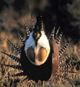
Sage Grouse image from Jessica Young's web site at: http://www.western.edu/bio/young/gunnsg/gunnsg.htm
Lecture 15, (20-Feb-13) Sage Grouse case history
Return to
Main Index page Go
back to notes for Lecture 14, 18-Feb-13
Go forward to notes for Lecture 16, 22-Feb-13
Required reading: Fujiwara and Caswell. Northern right whales. Nature (on WyoWeb)
Required reading: Kareiva. When one whale matters. Nature News & Views (on WyoWeb)
§§§§§§§§§
§§§§§§§§§§§§§§
§§§§§§§§§§§§§§§
§§§§§§§§§§§§§§§§
§§§§§§§§§§§§§§§§§
Let's look at some case histories of matrix-based analyses:
Sage Grouse in Wyoming case history:
Greater Sage-Grouse Centrocercus urophasianus are large game birds (males 3.2 kg, females 1.7 kg) that now occur in eight western states and two Canadian provinces.
Sage Grouse image from Jessica Young's web site at: http://www.western.edu/bio/young/gunnsg/gunnsg.htm
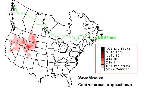
Fig. 15.1. Breeding Bird Survey data from USGS for Sage Grouse in North America.
Note that Wyoming is at the heart of the range. Birds on the Gunnison plateau in CO are now considered a distinct (and threatened) species. Web source: http://www.mbr-pwrc.usgs.gov/bbs/htm96/htmra/ra3090.html
Matt Holloran did his Ph.D. degree on the dynamics of WY Sage Grouse. He and I developed a matrix-based model based on a salient feature of their natural history -- overwinter survival of females is greatly affected by whether or not they are caring for a brood. Females with broods suffer reduced overwinter survivorship. Note that all fertilities will be females per female (reflecting female demographic dominance). Matt's model has just three stages (not age classes), based on the reproductive status of females:
First-year birds (Node 1)
Broodless hens (Node 2)
Hens with broods (Node 3)
Here's the life cycle graph:
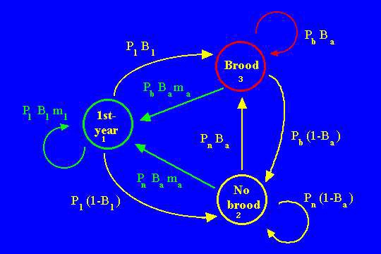
Fig. 15.2.Life cycle graph for female Greater Sage-Grouse. First-year birds can move to either of the two other stages, depending on whether their broods survive into the fall. A major distinction between the two "adult" stages is that broodless hens have higher overwinter survival (Pn > Pb, where Pb stands for survival of hens with broods and Pn stands for survival of hens with no brood). In addition to the normal Pi and mi terms, this formulation includes a term (another kind of vital rate) for the probability of being either with or without brood (Bi). Note that an arc connects every node to every other node; that is, the corresponding 3X3 matrix will be completely filled (all elements non-zero). The B and m terms have only two kinds of subscripts -- a for "adult" probabilities or fertilities and 1 for first-year birds. That is, we assume that a bird's fertility changes after the first year, but that a female's previous history of being with or without brood does not affect her future brood size (or her probability of being with or without brood late in the fall).
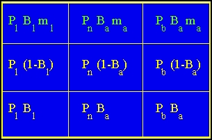
Earlier, I have shown the correspondence of the life cycle graph (the way you should formulate a model) to the matrix (the form in which the computer will analyze the model and compute eigenvalues and eigenvectors, etc.). We need to number the nodes in our life cycle graph. In a strictly age-classified model we have no choice (1 = first-year, etc.). For a stage-classified model the choice is sometimes arbitrary. It really doesn't matter whether "no brood" is Node 2 or Node 3. Once we decide, though, we have to stick with that because the numbering system will determine how we set up the rows and columns of our matrix. In this example, the first column will refer to arcs from the first node, second column to arcs from the second (no brood) node, and third column to arcs from the third (brooded) node. The rows will represent arcs to the given node numbers (e.g., all the first-row terms are flow to Node 1, or reproduction). Note that here we NEED to have aij with two subscripts -- we can't just rely on Pi and Fi, because we now have other kinds of transitions. This is not a Leslie matrix (which has elements only in the top row and subdiagonal). In fact, the matrix in Fig. 14.3 is completely full (no zero-value cells). That means that the corresponding life cycle graph has arcs each node and every other node -- it is possible to go to any node from every other node.
Fig. 15.3. Projection matrix corresponding to the life cycle graph of Fig. 14.2. The boxes in the top row are the fertility terms (green arcs in Fig. 14.2) for Node 1, Node 2, and Node 3. The other boxes are the transition rates between the various stages (yellow arcs in Fig. 14.2). These are some combination of survival (Pi) and probability of breeding (Bi) or not breeding (1 - Bi). The arcs go from the column to the row. That is the cell in Column 1, Row 2 (cell a21) corresponds to the arc from Node 1 to Node 2. Row 1, Column 3 corresponds to the production of chicks by hens that previously had a brood. And so forth....
Thoughts on parameterizing the model: Does it bother you that the broodless hens have a reproductive arc? Let's think about
1) the way we classify individuals, and
2) the time it takes to move along arcs between the nodes.
Consider the following hen. She fledges in August 2000 (we census her 1-Sep-00). July 2001 she lays a clutch but they don't make it. That sends her to the No-brood node. July 2002 she lays another clutch and they DO make it. She is doing that on her SECOND birthday. That gives her a reproductive arc (back from No-brood to Node 1). If we made her move to Brood first, she would be a full year older (2003) before she laid that successful clutch -- that would be her THIRD birthday, and not what we want. The only way we can have a No-brood to Brood transition with the correct time steps is by having the reproductive arc come out of the No Brood node. Standing in the middle of the census interval we could argue that the survival is determined by what Mom did in the past (she WAS a broodless hen with the higher Pn survival rate) but that she will now be moving to Brooded status (and that the future mi will only be credited to her if the chicks live long enough, after the next census, to reduce her next survival transition). Put differently, we can make it a requirement that we only give credit for mi if we will later consider that Mom bears a survival cost (Pb rather than the higher Pn) for that reproductive effort. These sorts of "what about this?" questions, and trying to wrestle with all the alternatives, are the only way to be reasonably sure that we have parameterized a model correctly.
This logic also helps answers the question about the possibility of having different P1 values. The P1 is survival from hatch (or fledging or whenever we census the chicks) to the first breeding season. They can't reproduce as fledglings, so they don't have a history behind them to affect their survival over the first year. So... not only do we not need to split up P1 by breeding status, we shouldn't.
The numerical values for the vital rates of Fig. 14.3 are:
0.259 0.672 0.560 0.338 0.390 0.325 0.112 0.210 0.175 Fig. 15.4. Numerical values for the cells of the projection matrix for Sage Grouse.
These vital rates (aij) describe probabilities of moving from one stage to another (both lower rows) or fertilities (the top row).
These sorts of numerical values are the basic input for most matrix-based demographic analyses.
We have taken two critically important steps in developing a demographic model:
1) We have formulated a life cycle graph that (we feel) captures the most important elements of the natural history. The distinction between hens with no broods and hens with broods is a (significant) difference in overwinter survival. If that is crucial, why not make that reproductive history the basis for the stages that make up the model?
2) We have translated the life cycle graph into a matrix that is ready for computer crunching. The computer program can take this 3X3 matrix and compute the eigenvalues, eigenvectors and, from those, all the interesting demographic correlates of the life cycle we have formulated.
Next, we'll turn directly to the sensitivity analysis (as we discovered in the take-home exam, we calculate the sensitivities as a cross-product of terms from the eigenvectors that describe stable stage distribution and reproductive values).
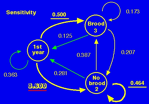
Fig. 15.5. Sensitivity graph for analysis of Sage Grouse life history, calculated from the matrix in Fig. 14.4. Each of the numbers is the sensitivity of l to a change in the given arc (arc in life cycle graph = element of the matrix). The three largest sensitivities are underlined and the largest is shown in shadow font with red underline. Note that, according to a sensitivity analysis, the two most important transitions in the life history are surviving through the first winter and surviving as a no-brood hen. This is in part because of the importance of any type of adult as a "reservoir" for the population. Note that l is much more sensitive to the overwinter survival of broodless hens than it is to the overwinter survival of hens with broods. One important management implication is that protecting or enhancing the overwinter survival of broodless hens may be the most effective management strategy for grouse. This could be especially important if broodless hens tended to winter in a different area or in different microhabitats than hens with broods. It might also be true that behavior (tendency to flock or not) could differ between brooded and broodless hens and provide a way to distinguish them that could then be used for setting management policies. We might have expected that protecting brooded hens would be the highest priority. The sensitivity tells us that our intuition might need some guidance from a demographic analysis. The sensitivity (sij, is the sensitivity of l to changes in the the arc from Node j to Node i) tells us the effect on l of an absolute change in one of the arcs. That is, we can tell, from the large value of 0.464 on the "No Brood" self-loop in Fig. 14.2, that an increase in the survival of broodless hens would have a large positive impact on l. The arc to which l is least sensitive is the production of offspring by hens that previously had broods (value of 0.125), the very transition that a biologist might reasonably have predicted as being most important.
In the graph below, we'll look at the elasticities. The elasticities assess the impact on l of a proportional change in the vital rates.
The sensitivities and elasticities tell us two things of practical importance to a manager or field biologist:
1) What transitions in the life cycle have the greatest importance to the population?
(Are the ones that are highly sensitive or elastic ones that we can do anything about in a management context?).2) What transitions should we measure most carefully in the field? What if the analysis tells us that adult survival is really important and egg production is relatively unimportant? Then the fact that we have clutch size estimates to the third decimal point may be irrelevant. BUT... if our survival data have wide confidence intervals, any conclusions we derive from our analysis will be tentative (because a small error in measure of survival rate would cause a large error in our estimate of l, for instance).
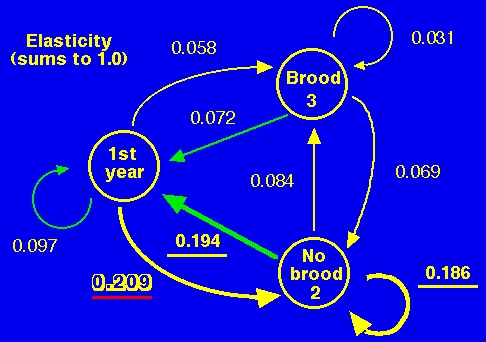
Fig. 15.6. Elasticity graph for analysis of Sage Grouse life history. Each of the numbers is the elasticity of l to a change in the given arc. The three largest elasticities are underlined and the largest is shown in shadow font with red underline. According to the elasticity analysis, the two most important transitions in the life history are becoming a broodless hen (arc from first-year to broodless) or producing offspring after overwintering as a broodless hen (arc from Node 2's No-brood back to Node 1), followed closely in magnitude by remaining a broodless hen (self-loop from Node 2 -- No-brood to No-brood). The shift from a sensitivity emphasis on Node1-Node3 to an elasticity emphasis on Node2-Node1 (offspring production by previously broodless hens) is due to the absolute magnitude of the original arcs (because the elasticity is simply the sensitivity weighted by the original arc coefficient and divided by l). B1is small, so e31 (which has B1 as a component) is reduced relative to the sensitivity arc, s31. In fact, e31 is the second smallest elasticity in the entire life cycle. The elasticity (eij) is the proportional sensitivity of l to a change in the arc from Node j to Node i. It tells us the effect on l of a proportional change in the arc (life history transition). Mathematically, the elasticity is the sij times the aij all divided by l, where the aij are the arcs in the original life cycle graph/matrix A, shown in Figs. 14.2, 14.3, and 14.4. That is, we weight the sensitivity (values in Fig. 14.5) by the size of the original arc (values from Fig. 14.4). One result is that l may be sensitive, but not elastic, to changes in an arc. An absolute change might have a big impact, but a proportional change won't because the original arc was so small. In monetary terms, a 1% change in your salary or mine has a lot less impact on the growth of the American economy than a 1% change in Bill Gates' annual earnings. In the elasticity analysis the least elastic arc (0.031) is the self-loop transition from brooded hen back to brooded hen. That is mostly because so few brooded hens manage to pull off a brood and make it back the next year. (i.e. the low a33 in Fig. 14.2/14.4 pulls the importance of that arc down when we move from sensitivity to elasticity).
An important assumption: sensitivity and elasticity analysis assess the impact of a small change in a vital rate. Any large changes require that we reformulate the matrix. This small-effect assumption is very similar to the assumptions underlying local stability analysis, where we assess the effects of a small perturbation's tendency to return to the equilibrium state (look back at the notes on stability analysis in Lecture 4).
Next, I will list some other outputs from the matrix analysis:
Mean age at beginning of stage (± standard deviation, s.d.)
Mean age of a stage is particularly interesting. Because time is implicitly a function of the analysis we can actually calculate a mean and variance of the age of individuals in each stage (the mean and variance are the first two moments of a distribution; we can calculate higher moments such as the skew and kurtosis as well). In the case of a very well-studied population of Florida Scrub-Jays with excellent demographic data, the ability to calculate mean age of a stage allowed at least partial validation of the model. Only if the calculated mean agreed well with observed values for each of the categories could we assume that the population was at equilibrium and that the model was correctly parameterized (of course, even if the data and model fit, that doesn't guarantee that the model is correct). The methodology for some very interesting age-based statistics from stage-classified matrices was developed by Cochran and Ellner (1992).First-year hens 0
Hens without broods 2.3 ± 1.8
Hens with broods 2.6 ± 1.9
Reproductive values, RVi (left eigenvector of the projection matrix, A)
First-year hens 1.0
Hens without broods 1.65
Hens with broods 1.38
Note that broodless hens have a higher reproductive value than do hens with broods. By definition, the reproductive value of the first stage is 1.0. One can think of the other numbers as being the "value" of an individual in other age classes, relative to the value of a first-stage individual.
Stable stage distribution, SSDi (right eigenvector of the projection matrix, A)
First-year hens 47.2%
Hens without broods 36.5%
Hens with broods 16.3%
(presented as % of total rather than the more usual proportions summing to 1.0) Note that broodless hens are almost twice as common as the brooded hens -- they are a major reservoir for the population's continued persistence.
Scalar product (SP): = 1 * 0.472 + 1.65 * 0.365 + 1.38 * 0.163 = 1.3
Summed lower level sensitivities (the lower level sensitivities are calculated via partial derivatives; they allow us to separate out the impact of the survival transitions from lower level terms such as the mi that go into compound terms such as Fi; remember, for example, that Fi = Pi * mi).
Survival terms (P) 43.5%
Probability of breeding (B) 38.6%
Probability of not breeding (1-B) 15.2%
Fertility (m) 2.8%Note that fertility is not a very important contributor to the total lower level sensitivity of l to changes in the life cycle.
Things that I still need to do:
What you need to know from this example:1) Assess the impact of environmental stochasticity on the conclusions drawn from the deterministic model developed here. Field effort devoted to accurate measurements of overwinter survival of hens is clearly merited.
2) Focus on particular transitions (component terms) that may be critical using techniques of:
Mark-recapture or other survival analysis methods
Variance and error estimators
I don't expect you to memorize any of the particular values or outputs of the material on the Sage Grouse. What I do expect is that you can follow through what each of the components is (e.g., what does a sensitivity mean?). I may, for example, present you with a similar analysis and ask you to interpret the output. Perhaps I would ask for the management implications. I might well ask what sorts of data a field biologist should focus on collecting carefully, given a preliminary matrix sensitivity analysis. A more difficult problem would be to find an inconsistency or mistaken parameterization in the formulation of a matrix model. That is, I might present you with a life cycle graph, and some "output" and ask "What's wrong with this analysis?"
Further web resources on Sage Grouse:
Jessica Young's Gunnison
Sage Grouse site:
Using a matrix-based population model, Fujiwara and Caswell (2002) were able to demonstrate that saving just one adult female per year within the population of endangered right whales could reverse the decline and cause a population increase. This could likely be accomplished simply by careful routing of ship traffic in the season in which females with calves are in major shipping lanes. I expect you to read the original paper and the News & Views overview by Peter Kareiva, so as to be able to answer the same sorts of questions as for the sage-grouse model.

A northern right whale. Fujiwara show that avoiding just one collision per year between a right whale and a ship could reverse the steady decline in this species. Females with calves are particularly vulnerable, because the calves need to surface for air more often.
§§§§§§§§§§§§§§§§§§§§§§§§§§§§§§§§§§§§§§§§§§§§§§§§§§§§§§§§§§§§§§§§§§§§§§§
References:
Fujiwara, M., and H. Caswell. 2001. Demography of the endangered North Atlantic right whale. Nature 414: 537-541. (On Reserve)
Kareiva, P. 2001. When one whale matters. Nature 414: 493-494 (News & Views overview of the Fujiwara paper. On Reserve)
Return to top of page Go forward to notes for Lecture 16, 22-Feb-13