Lecture notes for ZOO 4400/5400 Population Ecology
Lecture 16, (Friday, 22-Feb-13) Adding environmental
stochasticity to matrix-based models.
Return to Main Index page Go back to notes for Lecture 15, 20-Feb Go forward to notes for Lecture 17, 25-Feb-09
From deterministic to stochastic models.
Up to this point in the course all the population models we have considered have been deterministic. That is, we assume that the vital rates
(such as birth, death, immigration and emigration) are constant and unchanging over time. A single set of input values uniquely determines the
output values. The matrix models allowed vital rates to change with age or stage -- but they did so in a deterministic fashion.
We assumed that broodless hens or second-year individuals had unchanging vital rates year after year. One of the most obvious features of the real
world, however, is that the environment varies. One winter is harsh, the next is mild. One year is dry, the next unusually wet.
Such random variations in conditions are known as environmental stochasticity.
Every run of a deterministic model will yield the same (fixed) outcome. Every run of a stochastic model will vary, because we randomly alter one or more variables along the way.
What effect does stochastic environmental variation have on the conclusions
we have drawn by examining deterministic models? We will assess those effects by incorporating stochasticity in a matrix model, and
then comparing the results of multiple runs (simulations) with the fixed outcome of its deterministic equivalent.
We will start with a simple age-classified model with four age-classes. The life cycle graph is shown below.
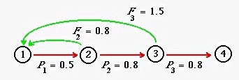
Fig. 16.1. Life cycle graph for an age-classified model with four age classes. The fertility arcs (green arrows) emerge
from Nodes 2 and 3, meaning that individuals do not reproduce as yearlings, but do reproduce in their second and third years. The fourth-year
individuals are present at the (post-breeding) census, but do not survive to reproduce at the next birth pulse. The values in this graph
will serve as the "base" graph/matrix for comparing a deterministic analysis with an analysis that incorporates stochasticity (via stochastically
varying the mi values).
If we run a deterministic matrix analysis of the life cycle shown in Fig. 16.1 (matrix A, with cells/arcs, aij)
we get the following outputs.
l (lambda) is 1.0000 -- we expect the population (at equilibrium)
to be stationary (neither growing nor shrinking).
Reproductive value vector, RV, with elements RVi is {1, 2.0, 1.5, 0}
Stable (st)age distribution (at equilibrium), SSD, with elements SSDj is:
0.451
0.225
0.180
0.144
(The cohort generation time, m1, is 2.6 years).
Sensitivities and elasticities will be important clues as to where environmental stochasticity will most strongly affect the
population dynamics. The sensitivities are the effect on l
of an absolute (e.g., + or - 0.01) change in a vital rate (aij). Remember that the sensitivity of l to a change in arc, aij, can be
assessed as the product of the reproductive value (RVi) of the node the arc is pointing to, times the stable stage distribution
(SSDj) of the node the arc is coming from (all divided by the scalar product, SP).
[Verbal definition of sensitivity - Value of target node, RVi, times size of source node, SSDj].
The elasticities are the proportional sensitivities -- effect on l of
a % change (e.g., + or - 1%) in an arc (vital rate, aij, such as an Fi or
Pi). We calculate them by multiplying the sensitivity of an arc (sij) by the original arc value
(aij), divided by l. The elasticity graph from the "base" life cycle graph
is:
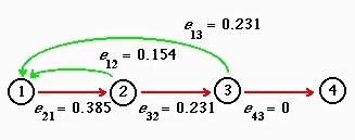
Fig. 16.2. Elasticities for the deterministic analysis of the life cycle graph shown in Fig. 16.1. Note that the arc to
which l is most elastic is first-year survival. In our stochastic
simulations we will be tweaking the less elastic fertility arcs (the green arrows).
[In order to incorporate stochasticity I use a general modeling program called Mathematica. Indeed, I use Mathematica for
most of the graphs, equations and calculations I use for producing the web pages for this course].
To assess stochasticity, we must conduct multiple runs, because the randomly varying input variable will make each run unique. Over
the course of a series of simulations, we can begin to see emergent patterns. Each run goes for 2,000 birth pulses (census intervals). At
each birth pulse, we left-multiply the projection matrix (with one or more cells slightly modified up or down by a random amount) against the
census vector (a vertical vector with the cells corresponding to the number of animals in each stage. Below I show the "base" matrix
corresponding to the life cycle graph of Fig. 16.1. The initial census vector consists of 10,000 individuals distributed in the proportions of the equilibrium
stable (st)age distribution (SSD). Each successive line shows the result of multiplying a slight random variant of the base matrix
against the current census vector. Notice that the only matrix value that changes is the P21 (first-year) survival arc. The four variants involve a "bad" year where survival went down, followed by three "good" years where it went up, with an average change
of ZERO (that is, the "good" and "bad" values, on average, canceled each other out).
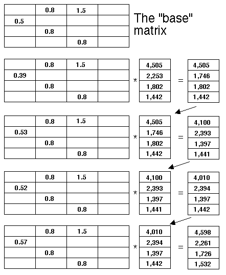
For each projection, I picked a random number that was slightly
larger or
slightly smaller than the "base" matrix's P1 value. On
the
first round the survival value went down a bit (from 0.5 to 0.39). That is, the only number that changes as we go down the sets is the lone number in the first column. And so forth....
Below is the output from 10 simulations, each of which ran
for 2,000
birth pulses. In other words, the calculations above could be
just
the first four of 2,000 squiggles in, for example, the red line below.
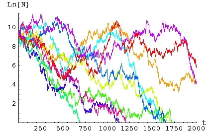
Fig. 16.3. Simulations of a matrix model with
stochastic
variation in the first-year survival rate. Each of the 10 simulations (differently
colored lines) ran for 2,000 birth pulses (years). Each
simulation
begins with 10,000 individuals distributed according to the
deterministic
stable age distribution given above. The Y-axis is the natural
logarithm of total population size, Ln(N) . The X-axis is time -- the
number of birth pulses or census intervals. Note that for this
series,
all 10 populations ended up with populations smaller than their
starting
size. Seven of the ten went (locally) extinct (hit the X-axis) before the end of
the
2,000 year period.
Conclusions: It certainly looks as though adding
stochasticity
has a detrimental effect on long term population size, and that this
effect
extends to the possibility of going extinct. [More extensive
simulations
would verify this preliminary conclusion].
Effect of varying the variation: The way I added
stochasticity was to add randomness to the first-year survival rate, P1. I did so by randomly
selecting the survival rate over each census interval from a beta distribution with a mean of 0.5 (the deterministic or "mean" value) and a standard deviation of 0.063. The probability density function (PDF) is shown in Fig. 16.4.
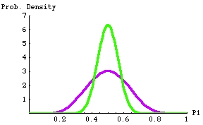
Fig 16.4. Probability density function (PDF) for beta distributions with mean at 0.5
(the
deterministic
value of P1). The difference in the variance (variability of the random draws) creates the difference
between the stochastic outcomes shown in Figs. 16.3 (severe negative impact) and Fig. 16.5 (more moderate negative impacts).
The lower, purple curve has a standard deviation (measure of spread of values around
the mean) of 0.125 (in the real world we expect the vital rates to vary around the mean).
The upper, green curve has a standard deviation of 0.063. Any particular random pick from either distribution will most
likely be near 0.6 (i.e., near the peak of the curve); it will be very unlikely to be below 0.35 or above 0.7 for the green curve,
and very unlikely to be below 0.2 or above 0.8. The beta distribution (in contrast to the normal distribution) has
the useful property that it is bounded by 0 and 1. That means we won't get survival rates that are negative or > 1
(which would not be biologically possible).
Reducing the "degree" of stochasticity (make the bounds of the ups and downs narrower).
Now let's see what happens if we do the same simulation
with one change -- cut the standard deviation in half for the stochastic variation in the birth rates (using the narrower green distribution in Fig. 15.4).
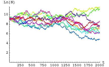
Fig. 16.5. Effect of reducing the standard deviation in
the stochastic fluctuations in a matrix model. The simulations are
the same as those conducted for Fig. 16.3 except that the standard deviation of the stochastic survival functions (P1)
is half the value used in Fig 16.3. Note that for this series, two of 10 populations ended up larger than its starting size, none went
extinct and the average size was considerably larger than in the "high variance" runs of Fig. 16.3. Nevertheless, even here, most
ending population sizes were smaller than their starting sizes. The difference between the outcomes shown in this plot and those
shown in Fig. 16.3 is driven by the difference in the variance of the survival rate (shown in Fig. 16.4).
Comparing Figs. 16.3 and 16.5 gives us further insights into the effects of stochasticity. With a lower variance, the long term population
sizes are larger. Lower variance "benefits" most populations.
Distribution of population sizes with stochasticity: A final note on the effect of stochasticity. Fairly complex analyses
of the effect of stochastic variation on long term matrix dynamics indicate that the asymptotic (meaning the value that an expression is headed
toward even if it never quite gets there) distribution of stochastically-driven
population sizes is lognormal (Fig. 16.6). That has some interesting implications for the expected population size across a set of
replicates (such as the sets of 10 we ran in Figs. 16.3 and 16.5).
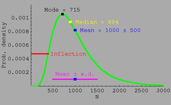
Fig. 16.6. Distribution of population sizes under stochasticity is expected to follow a lognormal distribution. The
lognormal has the property that the mean > median > mode. For the distribution shown, the mean population size is 1,000, but the
median is only 894 (meaning half the populations will be smaller than 894), and
the mode (the peak of the curve or most likely particular population
size in the distribution) is only 715. The tail of the distribution
goes way out the X-axis, meaning that a very low probability exists that a few populations will be extremely large (the distribution is skewed). A smaller variance (spread
of population sizes) would make the three mean/median/mode values more similar, but they would still have the relationship indicated above. A larger variance would increase the differences between mode, median and mean. Here, only 40% of populations will be expected to be larger than the mean value. Comparison to the normal (bell-shaped curve): with a normal distribution, mode, median and mean are exactly the same and the distribution is symmetrical.
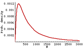
Fig. 16.7. Lognormal distribution with same mean as Fig. 16.6, but higher variance. Now the mode is only 171, and the median 555. For this distribution, only 29% of populations fall above the mean. The distribution is noticeably more skewed (higher peak and longer, more drawn-out tail).
The asymptotic lognormality of population size helps explain why the stochastic
runs shown above had values mostly lower than the starting size, even though the stochastic input was symmetric (Fig. 16.4). You might expect
that birth rates evenly distributed between larger-than-average and smaller-than-average
would even out and not adversely affect the long term dynamics of multiple runs. Not so.
Asymptotic lognormality means that as we do many (say thousands) of runs of a stochastic model (each running for 2,00 census intervals), the probability (Y-axis in the graph) of a given population size (X-axis) will approach the smooth shape of the curve above. Lots of values near the mode (~223) but a few very large values (shown by the long tail of the distribution, stretching out the X-axis).
Stochasticity has a net negative effect on population sizes -- a few populations may increase greatly, but most populations
will decrease in size, some may even go extinct. All this despite the fact that the "average" fluctuation will be zero (equal likelihood of
"good" and "bad" years).
• Question to ponder: the
results of the stochasticity analysis have some conservation implications. Think out at least one such
implication for management of threatened or endangered species.
Not required: See Chapter 14 of Caswell (2001) for more details and further references on incorporating
stochasticity into matrix models.
References:
Caswell, H. 2001. Matrix Population Models (2nd Edn.). Sinauer Associates, Sunderland, MA.
Emlen, J.M., and E.K. Pikitch. 1989. Animal population dynamics: identification of critical components.
Ecol. Model. 44: 253-273.
{Has some ideas for how to apply distributions to vital rates}
§§§§§§§§§§§§§§§§§§§§§§§§§§§§§§§§§§§§§§§§§§§§§§§§§§§§§§§§§§§§§§§§§§§§§§§
Return to top of page
Go
forward
to notes for Lecture 17, 25-Feb-13