Eqn 17.1
Lecture 17 (Mon. 25-Feb-13) Intraspecific competition
Return to Main Index page Go to movie of discrete logistic 2-cycle (r = 2.2) case Go to movie of discrete logistic chaos (r = 3) case
Go to movie of discrete logistic converge-to-K (r = 1.5) case
Go to back to lecture 16, Fri. 22-Feb Go to forward to lecture 18 of Wed. 27-Feb
In the previous lecture, we saw how environmental stochasticity could lead to fluctuating population sizes. In this lecture we will look at another possible cause of fluctuations in population size -- chaotic population dynamics -- driven by special conditions obeying a completely deterministic process.
Chaos has a specific mathematical meaning that is different from its everyday use in English. In everyday use, "chaos" implies an unpredictable lack of order. In the mathematical use, "chaos" means a process with extreme sensitivity to initial conditions and a tendency to wander around the set of possible values produced by a (deterministic) equation. Because it is deterministic, it has a high degree of order and predictability. The wandering may seem random, but it isn't. The tendency to spiral around zones of attraction (think of the valleys in the local stability cartoon of Lecture 4) leads to the kinds of fractal patterns that are popular for computer screensavers (see end of Lecture 17 for some of these fractal images).
Be sure you understand the difference between these two forces driving population fluctuations:
1. Matrix model with environmental stochasticity (randomness) -- populations size fluctuates (Lecture 16).
2. Discrete logistic equation (deterministic) with high r -- population size fluctuates (Lectures 17 and 18).
In both cases the population may seem to fluctuate irregularly, but the driving forces are entirely different.
The discrete logistic equation is deterministic (non-random). That means the equation predicts EXACTLY where the system/population size will go next. In the stochastic matrix case, we had random (stochastic) variation that drove the fluctuations. For the discrete logistic, two factors will drive the fluctuations:
i) a very high population growth rate (high r), plus
ii) the time lag introduced by using a discrete (time in "chunks" not continuous) formulation.
In the logistic model we saw how density could affect population growth. The way we incorporated that density dependence, was by introducing the concept of a "carrying capacity". The carrying capacity is largely internal to the population -- its own density is what causes the effect on population dynamics. As such, it is a result of intraspecific competition. This competition will manifest itself as density-dependent effects on the fertility or survival of some (or all) individuals in a population because of limited resources (such as food, space, access to mates, shelter). We will look at some of the mechanisms for competition among individuals, and then see how some of those mechanisms play out when we incorporate them into different kinds of models for population growth. By changing a few assumptions we can produce population patterns that are extremely surprising. We won't spend a great deal of time on INTRAspecific competition, but it will lead us into the next form of competition INTERspecific competition, involving populations of two competing species.
Before we begin incorporating intraspecific competition into different kinds of models, it is useful to consider some possible ways of classifying competition.
Two different ways of classifying major forms of competition:
I. Classification by access to resources
Contest -- winners and losers, Beverton-Holt curve, tendency to stabilize at K
emphasis on competitive ability (individuals responding to this form of competition are said to be K-selected)Scramble -- when shortage occurs everyone suffers, Ricker curve, can be very unstable (Hastings diagram)
emphasis on ability to colonize, high population growth rate
(individuals responding to this form of competition are said to be r-selected)
II. Classification by resource use pattern. How do individuals use resources?
Here is a table that compares and contrasts scramble and contest competition.Exploitation -- Individuals deplete the resource and make it unavailable
Interference -- Individuals control access to resources by dominance or territoriality.
Result may be that resources are abundant and undepleted.
Competition type Dynamics Equation Organisms Mechanism Growth rate Can be destabilizing Ricker Insects, marine fish Effects across age-classes High Stabilizing Beverton-Holt Vertebrates Strong within age-class effects Moderate
In what follows we will examine some extreme possible consequences of scramble and contest competition. Under some circumstances, scramble competition can lead to very surprising, destabilizing population dynamics. The appearance of these surprising dynamics, as generated by a very simple deterministic system/equation is one of the amazing discoveries of theoretical ecology in the last thirty years.
Strong contest competition, in contrast, will tend to act as a stabilizing force. This doesn't mean that scramble competition always leads to chaotic fluctuations, just that it can (if the population has a sufficiently high r value).
Lets look at some graphs that describe these two kinds of dynamics. The equation on which these are based is the discrete, difference equation form of the logistic given by:
Eqn 17.1
Compare and contrast this equation with the continuous, differential (meaning it has dN/dt) equation form of the logistic given in Eqn 5.1 (Lecture 5) whose solution (Nt as a function of t) we plotted as a smooth sigmoid curve (bounded by K) in Fig. 5.1. For the discrete logistic, time is "chunky" as opposed to smooth, analogous to the way matrix-based age-class (i) is discrete and chunky, as opposed to continuous and smooth age (x).
By changing the value of the growth rate, r, in Eqn 17.1 we can produce very different dynamic patterns.

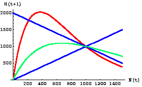
Fig. 17.1. Graph of population size, N, at time t+1 against population size at time t for Eqn 17.1. This diagram is called a "one-dimensional map" because it plots population size against itself (at different times). The carrying capacity, K, is 1,000 (the place on the graph where all the lines cross) -- it is an equilibrium point. Whether it is a stable or unstable equilibrium is determined by the slope of the colored (green or red) curves in the vicinity of the equilibrium point.
The shallow green line is a Beverton-Holt function describing contest competition (moderate r).
The steep red line is a Ricker curve describing scramble competition (high r).
Stability criteria (see Eqn 17.2, below): The straight blue reference lines have slopes of 1 and -1 (absolute values = 1). In the vicinity of K, curves with slopes that have
an absolute value less than one are stable (population number moves back toward K over time), while those with
an absolute value greater than one either oscillate or (if steep enough) show chaotic dynamics (do not return to K).
The green curve lies between the blue lines (absolute values < 1), so it has a stable equilibrium point.
The red curve lies outside the blue lines (absolute value > 1), so it has an unstable equilibrium point.
Note that the green line crosses the blue line with slope -1 only at the point {1000, 1000}, whereas the red line crosses at two other points (200, 1800} and {1800, 200}. [The latter point is offscreen to the right in this graph]. Those crossing points indicate the alternative states (combinations of population sizes) between which the population will oscillate.
Parameter values: red r = 2.7 (chaos), green r = 1.5 (stable), K = 1,000.
Try tracing a few numbers (or use Eqn 17.1 to calculate exact values).Chaos. For the red graph, starting at N((t)) = 400, the next nine population values are: 2021, 128, 1350, 525, 1893, 170, 1597, 319, 2006, 133. There is no discernible pattern to the sequence, and there are wild fluctuations (and the wild fluctuations never settle down, however long a series we calculate). The (deterministic) chaos results from the time lags (possible with a discrete formulation) and the very high r value.
Stability. For the green graph, in contrast, the population quickly converges on the carrying capacity (the stable equilibrium point that we found with the continuous, differential equation form of the logistic). Again, starting at 400, the next nine values are: 984, 1008, 996, 1002, 999, 1001, 1000, 1000, 1000, 1000 (once it reaches K it stays there).
The stability is determined by the slope of the N(t) vs. N(t +1) map equation's slope (m) in the vicinity of the "equilibrium" point, K. If the absolute value of the slope is greater than one
|m| > 1 Eqn 17.2
then the system will either oscillate or be chaotic. [The straight lines on each side of m are the mathematical symbols for "absolute value"]. The interplay between the blue lines above and the red or green lines delimit areas of stability (where |m|<1) vs. areas characterized by oscillations or chaos (where |m|>1. More explicitly, the green curve lies entirely within the triangle formed by the "arms and legs" of the X shape formed by the blue lines -- the triangle formed by the blue lines and the N(t +1)-axis on the left has its apices (meaning points; singular is apex) at {0, 2000}, {1000, 1000}, {0, 0}. The "triangle" on the right (open at the right beyond N(t) = 2000) has apices at {2000, 2000}, {2000, 0}, {1000, 1000}. Put differently, for N(t) < K=1,000 the green line is below the blue line with slope -1 and above the blue line with slope + 1. To the right of N(t) = 1,000 it is above the blue line with slope -1 and below the blue line with slope + 1.
Pushing the system to move from
1) rapid convergence toward K to
2) cycles to
3) chaos.
We can change the slope of the curves (and the dynamics/stability) by changing the values of r. The table below shows the ranges of r values that produce stability, cycles and chaos respectively.
Let's look at three "one-dimensional maps" with dynamics that range from stable (contest) to chaotic (scramble).

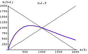
Fig. 17.2. One-dimensional map of the discrete logistic of Eqn 17.1 for an r-value of 1.5. Note that the slope of the curve in the vicinity of K (1000) has an absolute value < 1. It therefore has a single stable equilibrium point at K. The approach to equilibrium here will show damped or highly damped oscillations -- that is, the population will overshoot and undershoot a few or several times before settling at K. This is in the "contest" range for effects of intraspecific competition.

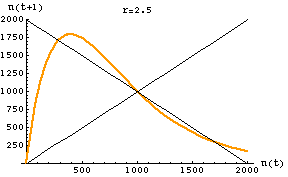
Fig. 17.3. One-dimensional map of the discrete logistic of Eqn 17.1 for an r-value of 2.5. Note that the slope of the curve in the vicinity of K (1000) has an absolute value > 1. The graph crosses the reference line in three places: 290, 1000, 1710. At K there is an unstable equilibrium. At the other two crossing points we find the stable equilibria for the two points the population will bounce between -- creating a two-point cycle. [It may take a while to settle on the equilibrium oscillation. Starting at a value of 400 it takes till the 134th iteration before it reaches and stays at the equilibrium values].
For a slightly lower r (2.2) with 2-cycle outcome see the first movie linked below:Go to movie of discrete logistic 2-cycle (r = 2.2) case Go to movie of discrete logistic chaos (r = 3) case
Go to movie of discrete logistic converge-to-K (r = 1.5) case
Fig. 17.4. One-dimensional map of the discrete logistic of Eqn 17.1 for an r-value of 2.7 -- the chaotic region. Note that the slope of the curve in the vicinity of K (1000) has an absolute value >> 1. The graph crosses the reference line in three places: N(t) = 214, 1000, 1786. At K there is an unstable equilibrium. The points 214 and 1786 will act as "attractors" but the population size will fluctuate wildly between limits somewhat above and below those points (my preliminary analyses suggest lower and upper boundaries at 127 and 2027). This curve is in the "scramble" range of effects of intraspecific competition.
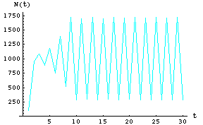
Let's look at the data of Fig. 17.3 (two-point cycle) through time.

Fig. 17.5. Plot of first 30 time steps for Eqn 17.1 with r = 2.5 (same r as in Fig. 17.3). Note that after some initial wandering the population exhibits a 2-cycle oscillation with a high of 1710, and a low of 290.
Compare that to the dynamics of a chaotic population over time.
Here are the breakpoints for r (for the interested)
Fig. 17.6. Plot of first 100 time steps for Eqn 17.1 with r = 3.5 (higher than Fig. 17.3 but also in the chaotic region of r values). Note that the population never shows any sign of approaching any sort of equilibrium.
Range of r Dynamic behavior 0 < r < 2.000 Stable equilibrium at K 2.000 < r < 2.526 Stable 2-point cycle 2.526 < r < 2.656 Stable 4-point cycle 2.656 < r < 2.685 Stable 8-point cycle 2.685 < r < 2.692 Larger-point cycles r > 2.692 Ch ao s
Question to ponder: what is the l (lambda)
corresponding to r = 2.692? Is that a high value?
What happens, even with very high r, if we run the discrete logistic with a starting population size of exactly 1,000?
What if we start with 1000.1?
A student once asked whether the places where the curve (one-dimensional map) crosses the downward linear m= slope of -1 line has any meaning. The answer is always "yes" and it's easiest to see under the special circumstances where r is between 2.0 and 2.526. Look at the crossing points in the graph below:
For other values of r, the interpretation is slightly less straightforward than for this two-cycle case. In the chaos region (r > 2.692), the crossing points will represent unstable equilibria that refer to "strange attractor" points -- places in the range of values around which the trajectories of the population tend to cycle. For lower values of r (< 2.0), the curve will cross only once at the single stable equilibrium point. For values between 2.526 and 2.692 the crossing points will be two of the several cycle spots.
Fig. 17.7. A population with an oscillatory population cycle due to density-dependent effects. The gold line crosses the black line whose slope is negative one in three places: an unstable equilibrium at K1 =K2 = 1,000 and two stable equilibria at the {X, Y} points {1,711, 290} and {290, 1,711}. [Note that the X-value of the first point becomes the Y-value for the second point and vice versa]. Once the population hits either equilibrium point it will continue to oscillate between those two population sizes indefinitely. In other words, it will bounce back and forth between a high of 1,711 and a low of 290 animals. Overshoot, semi-crash, overshoot, semi-crash etc.
Some highlights:
Introducing time lags can hugely change the dynamics. Moving from the continuous to the discrete logistic is a key to generating complex population dynamics. Changing from smooth time to chunky time makes chaos possible (because it introduces time lags -- by the time the population has gone through a time step it may have gone well beyond the equilibrium point K-- if r is large enough it will react by decreasing sharply; it will now oversteer to a very small size and so on, so that it never does get to the equilibrium point).
Under the right conditions (time lag via discrete driver, high r), simple deterministic systems can have complex dynamics. When biologists stumbled onto it (in the 1970's) it was extremely surprising (even to mathematicians) that a simple equation such as Eqn 17.1 could generate the sort of chaotic population fluctuations that we see in Fig. 17.6.
A defining characteristic of chaos is an extreme sensitivity to initial conditions. An infinitesimally small change in the starting conditions can produce a huge change in the result several time steps later, as we will see illustrated in Fig. 18.2 (Lecture 18 notes).
Very high growth rates (high r) (because they allow/cause overshoots) can lead to chaotic fluctuations.
Go to movie of discrete logistic 2-cycle (r = 2.2) case Go to movie of discrete logistic chaos (r = 3) case
Go to movie of discrete logistic converge-to-K (r = 1.5) case
References:
§§§§ §§§§§§§§§§§ §§§§§§§§§§§§§ §§§§§§§§§§§§§§ §§§§§§§§§§§§§ §§§§§§§§Beverton, R.J.H., and S.J. Holt. 1957. On the dynamics of exploited fish populations. Fishery Investigations 2: 1-533.
Bulmer, M.G. 1994. Theoretical Ecology. Sinauer Associates, Sunderland, MA. (Pp. 17-23)
Caswell, H. 1989. Matrix Population Models. Sinauer Associates, Sunderland, MA (pp. 231-233, 244-246).
Constantino, R.F., J.M. Cushing, B. Dennis, and R.A. Desharnais. 1997. Chaotic dynamics in insect populations. Science 275: 389-391.
Gurney, W.S.C., and R.M. Nisbet. 1998. Ecological Dynamics. Oxford Univ. Press, Oxford. (Pp. 125-129).
Hassell, M.P. 1978. The Dynamics of Arthropod Predator-prey Systems. Princeton Univ. Press.
Ricker, W.E. 1954. Stock and recruitment. J. Fish. Res. Board Can. 11: 559-623.
Return to top of page Go to forward to lecture 18 of Wed. 25-Feb