Eqn 20.1
Lecture 20 (Wed. 6-Mar-13) Analysis of interspecific competition by means of paired continuous logistic growth equations.
The Lotka-Volterra competition equations.
Return to Main Index page Go back to lecture 19 of Mon. 4-Mar Go forward to lecture 21 of Mon. 11-Mar
Download Excel demo of time-step analysis
When I discussed competitive exclusion I said that the most interesting case is when two competitors manage to coexist. We will now look at models for competitive coexistence using systems of paired logistic equations.
To work with a simple model of competition between two species we will return to a modified form of the continuous logistic equation (compare and contrast this with Eqn 5.1 of Lecture 5).
Eqn 20.1
where the subscript 1 refers to Species 1 and the 2 to Species 2. The g symbol (this is the Greek letter gamma) describes the nature of the competition between the species -- we will get to that in more detail shortly. Notice that if we took out the g12N2 term and removed the subscripts, we'd have the simple form of continuous logistic equation that we had in Eqn 5.1. Eqns 20.1 and 5.1 are forms of logistic growth that cannot overshoot the carrying capacity because the density dependence [= response to crowding] is instantaneous -- as opposed to the discrete logistic [Eqn 16.1] that we analyzed for the contest vs. scramble competition section. With the discrete logistic, overshooting and chaotic dynamics were possible because of time lags. Whereas Eqn 20.1 describes the dynamics of Species 1, a very similar equation describes the dynamics of Species 2:
Eqn 20.2
Let's look back at the interaction term gij. What the interaction term tells us is how strong an effect Species j has on growth of Species i, relative to the effect of i on itself. For example, if g12 = 0.1, then every additional individual of Species 2 has one tenth as much effect on Species 1 as would adding another individual of Species 1 -- that means that Species 2 doesn't have all that big a detrimental effect on Species 1.
Possible outcomes of the paired logistic equation model:
It turns out that the interactions described by Eqns. 20.1 and 20.2 have three possible outcomes:
1) Stable coexistence (both species persist, as in Fig. 20.1)What we will see is that the outcome depends on ratios of the carrying capacities, Ki, and the interaction coefficients gij. The way we will describe those ratios is by equations for inequalities such as those shown in Eqns 20.6. In order to examine the basis in inequality equations, we will conduct a stability analysis. As is often the case, we do so by setting the rate of change (dN/dt) to zero and solving the resulting equations. The additional complication here (compared to say the stability analysis of the single-species continuous logistic equation) is that we will be solving for the case where neither species has a tendency to change. Once we have established the stability criteria, we will look at some "cartoons" of population trajectories under various different initial conditions and differing combinations/ratios of the Ki and gij terms.2) Unstable coexistence (one species will "win" but which wins depends upon initial conditions or the direction of even the slightest perturbation from an unstable equilibrium for coexistence)
3) Competitive exclusion
a) Species 1 always wins
b) Species 2 always wins
Stability analysis -- where
does
the system have no tendency to change?
Let's say we have the following values for the
parameters
r and K:
r1
= r2 = 0.5, and K1 = K2
= 1000.
Assume also that g12
=g21 = 0.67. First, we'll set both equations to zero -- in other words, we
will ask "under what conditions will each of the species have no tendency to
change population size?" (we'll be doing a stability analysis).
Setting dN/dt in Eqns 20.1 and 20.2 to zero, we can
divide out the r1N1 term (start with Eqn
20.1; zero divided by r1N1 is
still zero) to yield:
Eqn 20.3
which simplifies to (the double arrows in the middle of each line mean that we are moving from one form of the equation to a rearranged or simplified version of the same equation):
Eqn 20.4
From equations to graphs --
plotting
isoclines (meaning lines of equilibrium or zero change). Eqn 20.4 describes a straight line on a plot of N1 against N2,
as shown in Fig. 20.1. [That is, Eqn 20.4
has the general form Y = b + mX]. The line
describes the value of N2 for which N1 is
at equilibrium (has no tendency to change -- but note that along
most of the line Species 2 will not be at equilibrium, so the size of N1 can be changed by changes in
N2). Let's look at the extremes.
If N1 is zero, then N2 will be at a Y-intercept value of
K1/g12 = 1,500. Along the other axis, N2
will equal zero when N1 = 1,000 (look at the left-most version of Eqn 20.4 to convince yourself
of that -- only when N1 = K1 will that
denominator go to zero). So we will have a line from a Y-intercept of N2 = 1,500
(=K1/g12)
to an N1 value of 1,000, as shown below. This line is
called the N1 isocline.
1) What is happening at {N1, N2 } = {1,000, 0}?
We SHOULD be at equilibrium because with no N2 around, the system boils down to Species 1 all by itself, which
(because it is just the "regular" logistic) has an equilibrium at K = 1,000.
2) Why an equilibrium at {N1, N2 } = {0, 1,500} which is the Y-intercept? Think of it this
way. Every 1.5 individuals of Species 2 "hurts" Species 1 as much
as 1 individual of Species 1 would "hurt" Species 1 (1/g12 = 1/0.667 =1.5).
All along the line connecting those two points we are just substituting one-and-a-half individuals of Species 2, for
every one individual of Species 1. {All along the red line in Fig. 20.1 we are just substituting more and more N2 as we
move up and left from the X-axis equilibrium point at K1}. The end point ({0, 1,500} is just the
place where an all N2 group have been substituted for the 1,000 = K1 individuals
that we had along the X-axis. That is, it takes 1.5 * 1,000
= 1,500 N2 to "make up" the effect produced at
the other end of the line by the 1,000 N1. Connect
those X- and Y-intercept dots and we have a line. That
(equilibrium) line is the red N1 isocline -- a linear equation describing N2 (Y-axis)
as a function of N1 (X-axis), as shown in Fig. 20.1.
Now do the same thing for Eqn 20.2 (i.e., set dN2/dt to zero) to get:
Eqn 20.5
(You should do the algebra to show that this
equation
is correct, by setting Eqn 20.2 to zero and then solving for N2).
This will be a line from N2 = 1,000 on the Y-intercept to N1 = 1,500 on the X-axis. This line is
called
the N2
isocline. In this case we
move from a "pure" single-species logistic (N2 only)
at K2 = 1,000 on the Y-axis to a spot where we
have 1.5 K on the X-axis (just Species 1 individuals).
{The reason I solved for N2 again
is that I want it to be in the form Y = b - mX}.
Now plot the two linear equations on a graph that shows the density of N1 against N2.
Let's look at the plot of the isoclines on a population size graph.
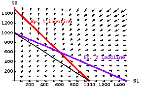
Vector field analysis. What are the arrow heads on this graph? They show the direction and strength of change for the two species analyzed jointly -- mathematically we do this by putting values into both equations at the same time and getting the change in the population sizes and then repeating that as many times as necessary to have the populations move to an equilibrium (stable coexistence or a "win" by one of the species). Start with the N1 axis. Given that N2 is zero, this reduces to the single species continuous logistic equation (Eqn 1.18). For N1 <K1 the population will grow; for N1 > K1 the population will decline, leading to an equilibrium at K1 = 1,000. On the N2 axis we see the same pattern. Near the origin, both populations will be increasing, so the vector points with an essentially 45° orientation. Anywhere above the red isocline, Species 1 will be tending to decline -- when we are near the bottom right, that decline will be the dominant force (with a slight tendency for Species 2 to increase when we are under its blue isocline). All together the arrows all point in toward the intersection of the two isoclines -- the stable equilibrium where neither species has a tendency to change size.

Fig. 20.1 Population plots for paired equations of continuous logistic population growth under interspecific competition. The red line depicts the isocline for Species 1 (dN1/ dt = 0 from Eqn 20.1, as solved in Eqn 20.4), while the blue line depicts the isocline for Species 2 (dN2/dt = 0 from Eqn 20.2 as solved in Eqn 20.5). The isoclines are given by Eqns 20.4 and 20.5. Note that the isoclines intersect at approximately N1 = N2 = 600. The thin black line connects the two carrying capacities and shows a total N1 + N2 = 1000 (K1= K2 = 1,000) --
I will refer to this line connecting the two carrying capacities as the " K-connector".
The fact that the isoclines cross above the K-connector line means that we have a greater TOTAL number of animals at equilibrium (1,200) than we would have if just one or the other species were present (1,000).
Parameter values inserted into Eqns 20.1 and 20.2: r1=r2 = 0.5; K1=K2 = 1000; g 12= g21= 0.67. The arrows represent a vector field analysis showing the size and directionality of two-dimensional population change.
Conclusion from Fig. 20.1 -- with values such that:
K1/g12 > K2 and K2 /g21 > K1 Eqns 20.6
stable coexistence is
possible
despite the interspecific competition
(i.e., despite the fact that the niches overlap). {We will add Eqns 20.6 to a
set of inequality "rules" in Eqns 20.1 that will delimit the major possible
outcomes of stable coexistence, unstable coexistence and competitive exclusion}.
Total carrying capacity. Note that the equilibrium point (intersection of the red and blue isoclines) is above the black line that shows a combined N1+N2 of 1,000. That means that with this kind of competition the total number of animals in the habitat is larger than the total if only one of the two species were present. {With curved isoclines, we could get a combined carrying capacity that was below the black combo. line -- we'll see examples of that later}.
We'll begin by redoing Fig. 20.1 as an animated cartoon.
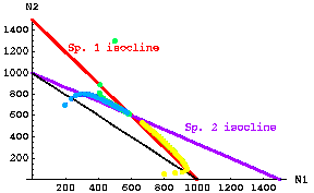
Below is an example of several starting points for Species1/Species 2 plots, and their trajectories over time toward the equilibrium for the case of stable coexistence. The yellow dots, for example, represent the path along which one of the dots in the "movie" moved towards the equilibrium point where the two isoclines intersect.

Fig. 20.2 Stable coexistence case. Trajectories through time for three different starting points of competition equations based on modified continuous logistic equations (Eqns 20.1 and 20.2). The three starting points were: yellow -- N1 = 800, N2 = 20; green -- N1 = 1,300, N2 = 500; blue -- N1 = 200, N2 = 700. Dots that are far apart represent very rapid movement; dots closer together represent slower rates of change (the time interval between dot "paintings" is constant, so fast rates make jumps, whereas slow change makes a smooth band). Note that the first green dot jumps very quickly to a value on the red isocline, then moves more and more slowly toward the equilibrium. Note also that the yellow trajectory takes a sharp corner. At first it moves quickly toward the red isocline (and N1 grows rapidly), then it follows the N1 isocline fairly closely toward the equilibrium point (so that N1 is decreasing).
Note the characteristic that the "visiting team" (N1) has a higher intersection with the Y-axis than the "home team" (N2). The "visiting team" (N2) is also further out the X-axis than the "home team's"K. The inequalities of Eqns 20.6 satisfy the conditions for stable coexistence.
Parameter values: r1 = r2 = 0.5; K1=K2= 1,000; g12 = g21 = 0.667.Go to "movie" of stable coexistence starting with low numbers of each species.
Go to "movie" of stable coexistence starting with 800 N1 and 50 N2 (the yellow arc in Fig. 20.2).
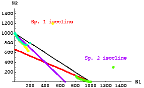
Here's a similar set of trajectories for the unstable equilibrium case.

Fig. 20.3. Unstable coexistence case. Trajectories through time for three different starting points of competition equations based on modified continuous logistic equations (Eqns 20.1 and 20.2). The three starting points were: yellow -- N1 = 500, N2 = 1,200; green -- N1 = 1,300, N2 = 400; blue green -- N1 = 200, N2 = 600. Dots that are far apart represent very rapid movement, those closer together represent slower rates of change. Note that the first yellow dot jumps very quickly to a value between the isoclines, then moves more and more slowly toward the equilibrium extinction of N1 and persistence of N2 at K2. Note also that the green trajectory takes a corner. At first it moves quickly toward the red isocline (and N1 decreases rapidly), then it follows the N1 isocline fairly closely toward extinction of N2 and persistence of N1 at K1.
Note the characteristic that the "visiting team" (N1) has a lower intersection with the Y-axis than the "home team" (N2). Likewise, the visitors (N2) have a less-than-K1 isocline crosspoint on the X-axis.
Parameter values: r1 = r2 = 0.5; K1=K2= 1,000; g12 = g21 = 1.5.Go to "movie" of unstable coexistence starting with 500 N1 and 1,200 N2.
Note that for the unstable case, if either species exceeds some threshold population size it will drive the other species to (local) extinction. N.B. that if the parameters (r, K, g) are exactly equal as in our simplest case then the species with higher population size "wins". If the parameters are not exactly equal, then the threshold ratio may be different from 50:50.
Conclusion from Fig 20.3: if
K1 /g12 < K2 and K2 /g21 < K1 Eqns 20.7
then the coexistence is UNSTABLE (the only parameters we have changed between Fig. 20.2 and 20.3 are the two gij values, BUT THAT CAUSES THE INEQUALITY SIGNS TO POINT IN THE OTHER DIRECTION). Thus, the inequalities of Eqns 20.7 satisfy the conditions for unstable coexistence. {We will add Eqns 20.7 to a set of inequality "rules" in Eqns 21.1 that will delimit the major possible outcomes of stable coexistence, unstable coexistence and competitive exclusion}.
What we have done in the material covered here is to find conditions under which different outcomes will occur. We have done so by means of a combination of equation-based analyses and graphical arguments.
Although we need to use the equations to solve the stability analysis, it is easier (at least for me) to use the graphs and some fairly simple rules-of-thumb to decide which of the three outcomes we have for a particular combination of r, K and g values.
§§§§§§§§§§§§§§§§§§§§§§§§§§§§§§§§§§§§§§§§§§§§§§§§§§§§§§§§§§§§§§§
Return to top of page Go forward to lecture 21 of Mon. 11-Mar