Lecture 21 (Wed. 13-Mar-13) Lotka-Volterra competition equations (continued).

Return to Main Index page        Go to back to lecture 20 , Wed. 6-Mar        Go forward to lecture 22 of Fr. 15-Mar  

Last time we used equations and graphical arguments to explore the conditions under which the Lotka-Volterra equations could produce outcomes of stable coexistence and unstable coexistence.  Now we'll look at the other major possible outcome -- competitive exclusion. 
{Here we have two subcategories -- Species 1 always wins or Species 2 always wins}.

Here's a graphical depiction of one of the two possible cases of competitive exclusion.

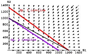
Fig. 21.1  Competitive exclusion of Species 2 by Species 1 (Species 1 "wins").  If the isocline of one population lies completely above the isocline of the other population, it will "win" from any starting point at which its abundance is > 0.  If the isoclines do not cross, no coexistence equilibrium exists, the only equilibria are all Species 2 (an unstable equilibrium, because as soon as N₁ >0, N₁ will increase to its K₁ and drive N₂ locally extinct), and all Species 1 (a stable equilibrium, because even if more N₂ show up later, the trajectories will move toward their local extinction).  Here, inequalities listed in Eqns 21.1 satisfy the conditions for a "win" by species 1.
Parameter values: r₁ = r₂= 0.5; K₁= 1,200; K₂= 1,000;  g₁₂ = 0.9; g₂₁ = 1.0.

Equation-based summary of outcomes:

Stable coexistence:  K₁ / g₁₂ > K₂ and K₂ / g₂₁ > K₁                                              Eqns 21.1

Unstable coexistence:  K₁ / g₁₂  < K₂ and K₂ /g₂₁ < K₁

Species 1 wins:       K₁ / g₁₂ > K₂ and K₂ /g₂₁ < K₁

Species 2 wins:       K₁ / g₁₂ < K₂ and K₂ /g₂₁ > K₁

Note that the inequalities above differ in that each has a different combination of > (greater than) and < (less than) signs.  The terms (which represent the X- and Y-intercepts for the isoclines) are exactly the same throughout.  That is, they make statements about the order in which the isoclines hit the N₁ and N₂ axes.

Likewise, it is usually much easier to look at "maps" of dispersion to decide whether a population is clumped, randomly distributed or uniformly distributed than it is to use analysis of counts per quadrat and the fit of the data to a Poisson distribution.  Nevertheless, the counts (frequencies, means and variances) are useful for quantifying the degree of clumping or uniformity, and for deciding whether a roughly random pattern is somewhat clumped or somewhat uniform. ____________________________________________________________________________________________________

How can we tell which outcome will occur, just by looking at the graphs?

IF the isoclines cross in such a way that the "visitor's" isocline hits the "home" species' axis above the "home team's" isocline, the coexistence is stable.  (Or, equivalently, if the isoclines are straight lines and cross above the K-connector, then we have the stable case).

IF the isoclines cross in such a way that the "visitor's" isocline hits the "home" species axis below the "home team's" isocline, the coexistence is unstable.  (Or, equivalently, if the isoclines are straight lines and cross below the  K-connector, then we have the unstable case).

IF the isoclines don't cross each other then whichever species has its isocline on top will outcompete the other species and drive it to (local) extinction. (Or equivalently, if the K-connector is between the isoclines and they do not cross it, then we have the competitive exclusion case).  [If most of the parameters (r_i and K_i) are equal, it will tend to be the case that g_i > 1 will give Species j an edge and lead to competitive exclusion of Species i (but see below)].

use the trajectory/vector method.  Above the N₁ isocline, N₁ will be declining (leftward arrow).  Below its own isocline N₁ will be increasing.  Above the N₂ isocline, N₂ will be declining (downward arrow).  Below the N₂ isocline, N₂ will be increasing (upward arrow).  IF the isoclines cross, they create four "regions":

1) Above both isoclines (leftward plus downward vectors yield a sum vector pointing SW);
2) above the N₁ isocline but below the N₂ isocline
            (leftward plus upward vectors yield a sum vector pointing NW);
3) below N₁ isocline but above N₂ isocline (rightward plus downward vectors yield a sum vector pointing SE);
4) below both isoclines  (rightward plus upward vectors yield a sum vector pointing NE).

Several good points about the vector sum technique:

a) It is quite general.  It also works well for graphical analysis of predator-prey equations
        and other paired equation analyses.
b) All you need to know to get started is

i) which isocline is which (a species own isocline goes to its K on its axis),
ii) that a species declines above its isocline and increases above it.

Some twists (potential pitfalls) in the Lotka-Volterra approach:

Stable coexistence case:

I. Stable coexistence but below K-connector: the effect of curved isoclines

Ayala et al. (1973) ran some interspecific competition experiments and had a puzzling outcome.  They found stable coexistence in some cases where the equilibrium point (intersection of the isoclines) fell below the K-connector.

Puzzling data:

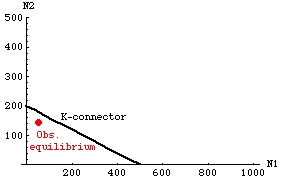
Fig. 21.2. Observed stable equilibrium numbers of two species of Drosophila following a competition experiment. Note that the combined population point (equilibrium) lies below the K-connector.

At first this seemed impossible, given the inequalities of Eqns 21.1. The stable coexistence outcome should have an equilibrium above the K-connector (see above). They carefully checked their empirically calculated estimates of K, and found that they were repeatable and precise. What they finally realized was that they had made an assumption of linearity for the isoclines -- the factors allowed by the model led inevitably to linear isoclines. Perhaps, the conclusion that "if the isoclines intersect below the K-connector, the coexistence is unstable" rule (see above) was simply an artifact of the model assumptions.

If the isoclines are linear and they cross above the K-connector, then yes, we have the stable equilibrium case. BUT, the isoclines can cross below the K-connector, and coexistence can still be stable, IF the isoclines are curved, as in the graph below. A slightly more complex model can produce curved isoclines, and curved isoclines are consistent with the observed isoclines.  When they monitored the population trajectories through time, those too were more consistent with a curved-isocline model than with the simpler linear model.

Fig. 21.3.  Stable coexistence with curved isoclines. Note that the isoclines cross below the K-connector. Nevertheless the intercepts satisfy the inequalities of Eqns 21.1 for stable coexistence -- that is, the "visitor" isoclines reach the intercept further out than the "home" isocline on both axes.  This modification of the original linear Lotka-Volterra theory (via slightly more complex equations 21.2 and 21.3) was developed to provide an explanation for experimental results with Drosophila.

Note that the vector sum method can accommodate this sort of change in the assumptions. Try dividing a sketch of curved isoclines into four areas and putting one arrow in each zone --
1) Above both isoclines (arrow points SW).  Both species decrease (toward equilibrium point).
2) Above Sp. 2 isocline, but below Sp. 1 isocline (the small area between the isoclines at values of N₂ between 200 and 300, near the N₂ axis). Arrow points SE toward equilibrium intersection of the two isoclines.
3) Above Sp. 1 isocline but below Sp. 2 isocline (long, very narrow area between the isoclines at values of N₁ between 500 and 800, near the N₁ axis). Arrow points NW toward equilibrium intersection of the two isoclines.
4) Below both isoclines (arrow points NE).  Both species increase (toward equilibrium point).

The model represented by Eqns 21.2 and 21.3 and Fig. 21.3 uses just a few additional assumptions and mathematical terms to allow us to fit a (relatively) simple model to real-world data.

For the interested (small blue font material): The curved isoclines result from using modifications of Eqns 20.1 and 20.2 with power terms:

                                   Eqn 21.2

                                 Eqn 21.3

All we have done to change Eqns 20.1 and 20.2 is to add power terms to the "home" species terms inside the bracket.  The power terms make the isoclines nonlinear.

II. Stable coexistence with gammas unequal and one of them > 1.0: Note that we can have a stable coexistence case even if one of the g_ij > 1.0. That is, what matter for coexistence are the inequalities given by Eqns 21.1. [Try these values to see a stable case with a g > 1]. Parameters: r₁ = 0.3; r₂ = 0.5, K₁ = 1,400, K₂ = 1,000, g₁₂ = 1.1, g₂₁ = 0.6].

Unstable coexistence case:

Parameters exactly equal, equal populations sizes (unstable equilibrium): Note that we can move along a very limited set of trajectories toward unstable coexistence under certain (very unrealistic) conditions. If the two species have all parameter values the same AND the population sizes are equal, they will move toward the intersection of the two isoclines and then have no tendency to move away. As soon as one or the other gains a numerical advantage, though, it will move toward its carrying capacity while driving the other to (local) extinction. Even if we start with N₁ > N₂ by just one animal, N₁ will "win". Conversely, if we start with N₂ > N₁ by just one animal, N₂ will "win". Any starting points that are not along that line will not move to the equilibrium point but will curve toward the "winner's" axis. [We could also create such linear trajectories in the more complicated case that the parameter values were not exactly equal. The result would still be a line going diagonally through the equilibrium point].

Ayala, F.J., M.E. Gilpin, and J.G. Ehrenfeld. 1973. Competition between species: theoretical models and experimental tests.
                    Theor. Pop. Biol. 4: 331-356.

Return to top of page                    Go forward to lecture 22 of Fr. 15-Mar