Eqn 23.1
Lecture 23 (Fr. 15-Mar-13) Predation (continued)
Return to Main Index page Go back to notes for Lecture 22, 13-Mar Go forward to lecture 24, 25-Mar-13
Last time I introduced the topic of predation (types, importance and indirect effects) and explored:
1) Mesopredator effects on birds in California scrublands
2) Functional and numerical responses and the case history of Bay-breasted Warblers as predators of spruce budworm
Now we will turn to the classic Lotka-Volterra equations for jointly analyzing predator and prey dynamics.
Why analyze predators and prey jointly?
It seems reasonable to expect that abundant prey lead to increased predator numbers and that the converse is true for prey. We will concentrate on just a couple of models. The first will be unrealistically simple.The Lotka-Volterra predator-prey equations/graphs (continuous, differential equations)
We will make the following assumptions:
Setting up the equations:Exponential growth of the prey in the absence of predation (like Eqn 4.5 and Fig. 4.5). [dN/dt = rV part of Eqn 23.1]
Linear functional response by the predator (more prey mean more eaten) -- remember we had a curved functional response in the Bay-breasted Warbler example (Fig. 22.1) [aV part of Eqn 23.1. Look back at Fig. 22.1 to check the units and the axes for the functional response]
Numerical response by the predator that is a constant times the functional response (tells us how prey consumption is converted into baby predators). Again, our previous numerical response example (Fig. 22.2) was a nonlinear curve. [b*(aV) part of Eqn 23.2]
Constant death rate of predators. [-dP part of Eqn 23.2]
{You may want to look at sections in the Gotelli text to get further info. on the concepts of functional and numerical responses by predators. We will return to, and modify, these responses in later analyses}.
We will give the victim population size (V) exponential growth minus a term due to predation loss.
Eqn 23.1
where r is the Victim population growth rate, aV is the functional response of the predator and
P is the predator population size.
The equation for Predator population size (P) is:
Eqn 23.2
where b is the constant that turns the functional response into a numerical response (i.e., consumption into babies) and d is the predator death rate. Note that if we take b(aV) as being a per capita birth rate of the predator, we could rearrange Eqn 23.2 to get:
Eqn 23.3
which is simply the equation for exponential growth, with P instead of N as the population size variable.
Solving for the isoclines:
We plot the dynamics in a manner very similar to what we did for the competition equations. We look for the conditions where population size will not change (an equilibrium point) by setting dSomething/dt to zero. In this case, we will set Eqns 23.1
(dV/dt) and 23.2 (dP/dt) to zero and solve for V or P. As for the competition equations, we use the resulting equations (23.4 and 23.5, below) to
draw isoclines (lines of equilibrium). Start with Eqn 23.1, the Victim equation, to find the number of Predators required to cause no change in the number of
Victims. We will call that equilibrium Predator number "P-hat", and write it as:
![]()
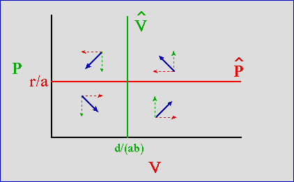
Because r and a are constants, the equilibrium value for the predators (resulting in no tendency for V to change) will be a straight line, perpendicular to the Predator axis (which is the Y-axis in Fig. 23.1). When we have a value of P higher than r/a the victims will tend to decline (more Predators eat more Victims); values of P below the r/a line will cause victims to increase (fewer Predators eat fewer Victims).
Eqn 23.4
Do the same for Eqn 23.2.
Eqn 23.5
again, d, a and b are all constants, so we'll have a straight line perpendicular to the Victim axis (the X-axis). If the V are greater than the line d/ab, it will cause predators to increase (more food converts into babies). V less than the line d/ab will cause predators to decline. We can put these all together on a graph.
Graphing the isoclines and using vector-sums to indicate joint trajectories:
Here's the graph for the predator-prey isoclines. Note that I use the vector-sum method to outline the dynamics of the four zones created by the isoclines.
The graph above hints at population cycles -- the prey shoot up, the predators then increase, the prey crash, the predators then crash and the prey then shoot up again.

Fig. 23.1. Predator-prey phase plot (prey, V, on the X-axis, predator, P, on the Y-axis. The predator's isocline is the green vertical line, labeled V-hat -- when prey are more abundant than d/ ( ab) the predator increases (upward dashed arrows). When the prey are below d/ ( ab) the predator declines (downward dashed arrows). The prey's isocline is the horizontal red line, labeled P-hat-- with more than r/a predators the prey decline (leftward dashed arrows). When predators are below r/a, the prey increase (rightward dashed arrows). If we sum the vectors for predator and prey trajectories (angled, solid blue vectors) we see that they tend to orbit around the equilibrium isocline intersection.
Phase plot of the joint trajectories:
How would we go about calculating the joint trajectories of predator and prey? That requires solving the following differential equation:
Eqn 23.6
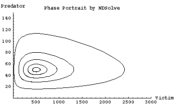
(Note that Eqn 23.6 is simply the left-hand sides of Eqns 23.1 and 23.2 on top of each other, with the dt parts canceling). Solving Eqn 23.6 requires the technique called "separation of variables." (I used separation of variables to solve dN/dt = rN for N in Eqns 4.6 to 4.12, and again to solve for N with the logistic equation). Even with the solution via separation of variables we have an indefinite integral that cannot be solved explicitly -- because two solutions exist for every X-value, and two for every Y-value (as shown in the loop form of the trajectories in Fig. 23.2, below). Our competition trajectories didn't go round in orbits this way. We need to resort to numerical techniques, including what are called interpolating functions. The mathematics for doing so is beyond the scope of this course. (A computer program such as Mathematica can do most of the grunt work for us). The resulting phase plot is shown in Fig. 23.2.
The behavior shown by Fig. 23.2 is sensitive to/dependent upon initial conditions. Previously, with our competition equation analyses, many different initial conditions would converge on a single equilibrium point (either stable coexistence or extinction of one or the other of the two species). Here, in contrast, every initial condition will have its own closed loop around which it cycles endlessly. A "movie" of the trajectories would show dots moving around each of the loops above in endless cycles. The outer loops will take longer to go all the way round and speeds will change in different parts of the loops (e.g., fast predator crashes on the left-hand edge of the outermost egg-shaped trajectory).

Fig. 23.2. Phase plot of predators against prey with isoclines like those of Fig. 23.1. Any initial condition (point in the phase plot representing the joint abundance of predator and prey) lies on a closed loop that will cycle in the same orbit (i.e., come back to its initial condition on each cycle). Each of the loops in the figure therefore results from a different initial condition. The outside loop started at {V = 20, P = 50}, the next at {120, 50}, then {220, 50}, {320, 50} and the innermost loop started at {420, 50}. The amplitude of the cycle (difference between maximum and minimum values) therefore depends upon the size of the initial deviation. Only an initial condition of {500, 50} would stay at the point of intersection of the two isoclines (because that is the equilibrium point that is the focus for all the orbits). Note that the trajectories are not circular because the prey grow more quickly than do the predators (maximum prey abundance is 5 times equilibrium, whereas maximum predator abundance is three times equilibrium). The cycle is: prey explosion, prey crash, predator crash (with a slower rise in the predators happening along the "width" of the egg-shaped orbit). Note that for these parameter values, and starting with just 20 prey as the initial condition, the predator crash occurs along a line that is very close to prey extinction.
Parameters: r = 0.5, a = 0.01, b = 0.2, d = 0.1. [Check these parameters against the isocline solutions of Eqns 23.4 and 23.5].
I calculated the trajectories with Mathematica routines, aided by the Mathematica-based book: Gray, A., M. Mezzino, and M.A. Pinsky. 1997. Introduction to Ordinary Differential Equations with Mathematica. Springer-Verlag, NY and its ODE.m package.
Summary of Lotka-Volterra system of Eqns 23.1 and 23.2:
• Simple (unrealistic) assumption of exponential growth of prey in absence of predator (term rV in Eqn 23.1)References:• Simple (unrealistic) assumption of linear functional response of predator to prey density (term aV in Eqn 23.1)
• Simple (unrealistic) assumption of linear numerical response of predator
(conversion of prey into baby predators -- term b(aV)P in Eqn 23.2.• Cyclical behavior of predator and prey densities (reasonable)
but cycle amplitude determined entirely by initial conditions (unreasonable).
Bulmer, M.G. 1994. Theoretical Ecology. Sinauer Associates, Sunderland, MA.§§§§ §§§§§§§§§§§ §§§§§§§§§§§§§ §§§§§§§§§§§§§§ §§§§§§§§§§§§§ §§§§§§§§Gray, A., M. Mezzino, and M.A. Pinsky. 1997. Introduction to Ordinary Differential Equations with Mathematica. Springer-Verlag, NY.
Gurney, W.S.C., and R.M. Nisbet. 1998. Ecological Dynamics. Oxford Univ. Press, Oxford.
Return to top of page Go forward to lecture 24, 25-Mar-13