Lecture notes for ZOO 4400/5400 Population Ecology
Lecture 24 (Mon. 25-Mar-13) Predation (continued)
Return to Main Index page
Go back to notes for Lecture 23, 13-Mar
Go forward to lecture 25 , 27-Mar-13
Last time I introduced the classic Lotka-Volterra equations for jointly analyzing predator and prey dynamics. The basic model makes some rather unrealistic simplifying assumptions.
Can we do better? The Lotka-Volterra predator-prey model is what is called "structurally
unstable". That means that if we tweak parameters a little (e.g., by changing the starting population sizes, which we call the
"initial conditions") then we get very different outcomes. We would like our model to be a little more robust
(less sensitive to initial conditions and less sensitive to reasonable changes in the assumptions).
First "improvement" -- logistic prey growth. Let's see what would happen to the system if we made one reasonable
improvement in the predator-prey model. We will include density -dependence for the prey. Our approach will be
graphical -- that is, rather than try to solve increasingly complex equations, we will make inferences about
the system's behavior based on examination of graphs for a variety of shapes and placements of the isoclines.
Again, the vector-sum method will be a very useful tool.
Intraspecific competitive effect. What would a density-dependent (logistic-based) prey isocline look like? Most
obviously perhaps, we'd expect the prey growth rate to decline at high levels of its own population, V.
That "crowding" effect would pull the right-hand side of the red isocline in Fig. 23.1 downward.
Interspecific predator/prey ratio effect. The "equilibrium" predator-prey ratio is 1:10 using the parameters in Fig. 23.2 (the bull's eye is at P = 50, V =500). What if we have an excess of the predators relative to prey
(e.g. ratios like 2:10 or 3.1:10)? Excess predators will eat more prey, and reduce prey numbers. The result will be to pull
the left-hand side (LHS) of the prey isocline downward, also.
The result of the combination of intraspecific competition (pulling down RHS) and excess predation (pulling down LHS)
will be a "humped" prey isocline.
With a "humped" prey isocline we have two qualitatively different places we could place the vertical predator isocline (we
won't change the predator isocline for the moment).
Left of the hump
Right of the hump.
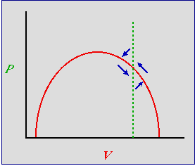
Let's start to the right of the hump, as shown in Fig. 24.1.

Fig. 24.1. Predator-prey phase plot incorporating density-dependence for the prey -- with predator isocline to the right
of the hump. An inefficient predator -- prey occur at high densities
at equilibrium. Red solid curve: prey isocline; green dashed line: predator
isocline. Blue arrows are the summed predator and prey vectors, as in Fig. 23.1
Note that the blue arrows all point at one or more isoclines, leading to stability.
What has this done for us? The two most important blue arrows in Fig. 24.1 are the one pointing NE and the one pointing SW.
Imagine that we start (initial condition) at the bottom of the arrow pointing NE. In contrast to Fig. 23.1
we are quite close to the prey isocline -- that is, the prey will start declining again, even before we have reached the equilibrium predator
density. Now continue on to the arrow pointing SW. Again, in contrast to Fig. 23.1 we are close to the prey isocline --
they begin to increase even before the predator has declined to its equilibrium density. That will reduce
(actually eliminate) the severity of the "crash" that we see on the left-hand side of the trajectories in
Fig. 23.2 . The behavior of the system has changed. Now, instead of sensitive
dependence on initial conditions, many different starting points will all tend to spiral inward to the same destination --
a stable equilibrium at the intersection of the isoclines.
Density-dependence for the prey and inefficiency of the predator combine to
stabilize the system.
Question to ponder: In this stability analysis, we will restrict our attention to
perturbations near the equilibrium. What similar sort of assumption-for-the-purpose
of stability analysis did we make when considering matrix models?
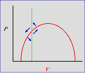
Now let's try the predator isocline to the left of the hump.

Fig. 24.2. Predator-prey phase plot incorporating density-dependence for the prey -- with predator isocline to the left
of the hump. An efficient predator -- predator keeps prey at low densities at equilibrium. Red solid curve: prey isocline; green dashed
line: predator isocline. Blue arrows are the summed predator and prey vectors, as in Fig. 23.1 and Fig. 24.1. Note that the blue
arrow pointing SW does not point toward an isocline but toward the Y-axis (prey extinct) or even the origin (both extinct).
The result is instability (a tendency for the the predator and prey to crash). Also, the arrow pointing NE
parallels the isocline so that it does not cross it near the equilibrium point.
From stable to unstable. What effect does this change in placement of the isocline have? Again, the two most
important arrows point NE and SW. Again, start at the bottom of the NE arrow. In strong contrast to Fig. 24.1 (and even worse
than Fig. 23.1) the vector doesn't reach the prey isocline
until we are above the predator equilibrium. The prey are really overshooting and will provide plenty of food for predator growth. Now look at the SW
arrow. We've got lots of predators and the prey isocline isn't even in the "line of fire". The predator will crash and the vector will turn
only when the predators have virtually disappeared. The system is actually less stable than the simple (straight-line) Lotka-Volterra system of
Fig. 23.1. An efficient predator is one that is able to keep its population growing, even when the prey are at low
densities -- the prey have little or no refuge from predation.
Effect of shifting the predator (V-hat) isocline. What is the major difference between the models of
Fig. 24.1 and Fig. 24.2? Efficiency of the predator.
Whether the predator isocline falls to the left or to the right of the prey isocline's hump is determined by the
efficiency of the predator.
An inefficient predator can't really keep the prey in check -- indeed prey density may
be determined in large part by its own carrying capacity. Further, if the prey are at low densities, the predator will start to
decline (easing pressure on the prey). We will tend not to have dramatic boom-crash cycles.
In contrast, the model of Fig. 24.2 implies an efficient predator. In this case, the
prey are kept at low densities by the predator -- with the unstable consequences
we examined above. By the time the predator begins to decline, the prey are at very low density, tending to cause a predator crash.
Adding threshold density-dependence for the predator. Now let's think about some possible isocline shapes for the predator
that also incorporate a little more realism than the straight-line isocline of the basic Lotka-Volterra equations (Eqns 23.1 and 23.2). At low
predator density we will continue to use the sort of linear numerical response that we had earlier. At high predator densities however,
we will incorporate a threshold effect for the predators -- at some critical density they interfere
with each other, use up all the available (and necessary) territories or dens, or have some other sort of negative effect on each other. That
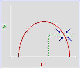
will cause the predator isocline to take a sharp bend to the right, as shown in Fig. 22.5.

Fig. 24.3. Predator-prey phase plot incorporating density-dependence for the predator as well as the prey. Red solid
curve: prey isocline, P-hat; green dashed line: predator isocline, V-hat.
Blue arrows are the summed predator and prey vectors, as in Fig. 23.1. Note that the blue vector sum arrows no longer
have a cyclic pattern. Now they all point inward toward the stable equilibrium. The result is a locally
(near equilibrium) highly stable system -- any deviation will have a strong tendency to return to the
equilibrium point.
The result is a system that is even more clearly stable. Look at the arrows now -- they all point straight in toward the
equilibrium.
We have learned several lessons about modeling dynamics:
1) Even fairly simple sets of equations can have complex dynamic solutions that can require advanced numerical
techniques to plot the trajectories -- and results in cyclic oscillations in predator and prey
densities.
2) The simplest Lotka-Volterra system is structurally unstable.
Structurally unstable means that the dynamics are
heavily dependent on the details of the initial conditions.
Each particular combination of predator and prey will have its own
egg-shaped orbit, as seen in
Fig. 23.2.
3) With density-dependence for the prey, the stability depends upon where the predator isocline crosses the prey
isocline.
A system with an inefficient predator will tend to be fairly stable. A system with an
efficient predator will tend to be unstable.
4) The addition of density dependence for both prey and predator strongly stabilizes the system.
5) Graphical techniques can sometimes provide qualitative answers to problems that are
mathematically difficult.
All of the analysis for Figs. 24.1 to 24.3 relied on qualitative graphical analysis rather than the details of
equations.
References:
Bulmer, M.G. 1994. Theoretical Ecology. Sinauer Associates, Sunderland, MA.
Gray, A., M. Mezzino, and M.A. Pinsky. 1997. Introduction to Ordinary Differential Equations
with Mathematica. Springer-Verlag, NY.
Gurney, W.S.C., and R.M. Nisbet. 1998. Ecological Dynamics. Oxford Univ. Press, Oxford.
§§§§
§§§§§§§§§§§
§§§§§§§§§§§§§
§§§§§§§§§§§§§§
§§§§§§§§§§§§§
§§§§§§§§
Return to top of page
Go forward to lecture 25, 27-Mar-13
