Eqn 15.1
Return to Main Index page Go to Lecture 16 Go to Lecture 17
Go to movie of discrete logistic 2-cycle (r = 2.2) case Go to movie of discrete logistic chaos (r = 3) case
Intraspecific competiton -- discrete logistic equation
low
r slightly oscillating approach to K case
Embedded QuickTime Movie (from Mathematica notebook r1Movie.nb)
Click on the image below to start the "movie". A control bar will appear below the graph; the various buttons will allow you to stop and start it.
Fig. 1. One-dimensional "map" of the discrete logistic (Eqn 15.1, above) with r = 1.5 and K = 1,000. Note that the population converges very quickly on K. We start with an N(t) value on the X-axis, move up to the "map" (red line) to get an N(t+x) value and then take the corresponding Y-value by going over to the 1:1 black line, then again move to the red line. Tracing the map is therefore a process of going back and forth from the red map line to the black N(t+x) = N(t) 1:1 line (like a stair step -- "up, over, up, over"). Following the map this way gives us the successive population sizes over time. Note that the trajectory moves toward the stable equilibrium point (at K = 1,000). The last few frames involve changes so small they don't show up onscreen.
The low r value here is what permits the convergence on K.
Return to top of page
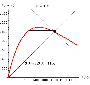
Fig. 2. Static view of the trajectory toward the stable equilibrium at K = 1,000 from a starting N0 of 120.
Note the stair step ascent from the starting value to K. The very slight oscillations are shown by the lines spiralling inward around K.