Lecture 10, (Wednesday, 6-Feb-13)

Sex ratios, Natality

Return to Main Index page     Go back to notes for Lecture 9,  4-Feb      Go forward to notes for Lecture 11,  8-Feb

What other demographic aspects of populations might we want to consider besides their survival and mortality rates? At least two other features are sex ratio and age structure (age ratios).  Each of these can affect population dynamics in interesting ways or provide clues about forces shaping those dynamics.  Let's look first at sex ratio -- the ratio of males to females.

Sex ratio

Sex ratio can have important effects on population dynamics.  We will consider some of the forces that act to change sex ratios as well as broad patterns of sex ratio variation n the animal kingdom.

Sex ratio is the proportion of males relative to the proportion of females. It can be expressed in several ways, some of which are shown in the table of equivalents below:

Ratio        Male: female	Proportion males	Percentage males
50:50	0.5	50%
2:1	0.67	67%
3:1	0.75	75%

As we move across rows in the table we are expressing the same sex ratio in different ways. As we move down the columns we are changing the sex ratio (toward more males) but using the same notation. Another, verbal way of expressing the sex ratio is to say that it is "male-biased" (more males than females) or "female-biased" (more females than males).

Ernst Mayr classified sex ratios according to the stage in the life cycle:

Primary sex ratio: sex ratio at conception (the point at which the sperm fertilize the eggs). This is usually near 50:50 in natural populations, though a few cases exist where parasites can change the primary sex ratio by for example, having lethal effects on sperm.

Secondary sex ratio: sex ratio at time of hatch or birth. Often nearly 50:50 but more examples exist of skewed secondary sex ratios than of skewed primary sex ratios.

Tertiary sex ratio: sex ratio at some later stage of life such as at age of first reproduction or "adult" stage. Skewed sex ratios are most often observed at this stage.
            [Some authors distinguish between tertiary (juveniles) and quaternary (adults), but we won't worry about that distinction]

Two generalities emerge from the broad patterns we have considered above:

1)  Sex ratio skew tends to become more pronounced at later stages. For example, primary sex ratios seem rarely to differ much from 50:50, secondary sex ratios can vary slightly more and we most often find skew in tertiary sex ratios.

2) Bird pattern differs from mammal pattern. Avian tertiary sex ratios seem generally to be skewed towards males, tertiary ratios of mammals tend to be biased towards females. Let's look at some data:

The following table shows both a change in sex ratio (away from 50:50) with age, and a difference between birds and mammals in the direction of the bias. The three mammals at the end of the table all show a bias towards females. The birds show the reverse.

Examples of ungulate sex ratios. Note the increasing bias toward females in the elk data (which are the only data for prenatal ratios):

So, the empirical data show that adult sex ratios in birds often tend to be male-biased, while those in mammals tend to be female-biased.

What might explain this pattern of sex ratio differences between birds and mammals?  Let's look at three apparently plausible alternative hypotheses that might explain the pattern.

Hypothesis I. The "chromosome" hypothesis

Hypothesis II. Density-independent mortality (predation, physiological stress) hypothesis

Hypothesis III. Intraspecific competition hypothesis

Hypothesis I. The "chromosome" hypothesis (higher mortality in the heterogametic sex)

Heterogametic sex (in species with chromosome-derived sex determination, the sex that has the "different" chromosome is called the heterogametic sex).

Mammals:   Male XY, Females XX

Birds:          Males ZZ Females WZ

Recessive deleterious alleles can have more effect in the heterogametic sex because of expression of recessive alleles. A recessive allele is a form of a gene that is expressed only when it occurs in a homozygote (an individual who has both copies of a gene the same)-- when it occurs in a heterozygote it is blocked by the other "dominant" allele.  For XY males, a recessive allele on either chromosome will be expressed just as if that individual were a homozygote (the Y or X chromosome won't carry the alternative allele that would compensate for the harmful allele).  A related phenomenon appears in the context of hybridization. Haldane's Rule holds that hybrid sterility will be more common in the heterogametic sex.

Hypothesis II. Density-independent mortality (predation, physiological stress; could drive ratio either way, depending on which sex suffers greatest stress)

a) Reproduction related stresses

Female birds on nests: may be much more vulnerable on the nest than normally. 
(What about birds in very protected nest sites, such as burrows or cavities?)

Polygynous male mammals: males may expend so much energy on attracting or defending mates that they are more vulnerable to predation or their condition deteriorates.  

b) Dispersal-related risk (higher mortality in dispersing sex)

Female dispersal in birds (Florida Scrub-Jay females move three times as far away from where they hatch as do males)

Male dispersal in mammals

Example: Richardson's ground squirrel sex ratio goes from 50:50 to 11:89
Why? Young males 1) start hibernation late, 2) emerge early, and then 3) are driven off by females and dominant males. Each of those three factors raises the risk of predation. Mt. Lions, bears, other carnivores may also show same pattern of greater dispersal by males with associated risks.

Hypothesis III. Intraspecific competition (depends on which sex is dominant in contests for resources)

Dominance status may affect condition and survival: Pheasant sex ratios on Protection Island became more male-biased as density increased. Males appeared to be able to gain priority access to resources important to survival because of their larger size.

Winter ranges may be different.

Bull elk may winter in areas of deeper snow. [Males at greater risk]
Female Wilson's Warblers migrate much further south (southern Central America) because males migrate first and take all the best spots in the northern end of the wintering range (Mexico). [Females at greater risk].

Male mammals (in species where males are larger than females) may have higher energetic requirements because of larger body size and be more vulnerable to food shortages. Where males are larger but can't keep others from the resource (e.g., with highly dispersed grazing resources) then larger size can be a detriment to survival in harsh conditions.

  I mentioned the St. Matthews Island AK reindeer introduction and crash earlier in the course. What I didn't say anything about was which animals died.  Here are the numbers
         1944: 29
         1963: 6,000
         1964: 42 (but only one was male!)
              1:41 sex ratio.

How can we discriminate among these three alternative hypotheses? Unfortunately many of the predictions arising from the hypotheses are not mutually exclusive. That means they could ALL be playing a role, and the best we might be able to do is provide supportive evidence that suggests a larger role for one of them. We might, for example, use "exceptions to the rule" to test the strength of a hypothesis.

Example # 1 of a predictive test. Say polygynous vs. monogamous rodents (e.g., the polygynous meadow vole Microtus pennsylvanicus versus the monogamous prairie vole M. ochrogaster) showed an even sex ratio in the monogamous species, but a female-biased sex ratio in the polygynous species. Say also there was no difference between the species in dispersal or density, then we'd have support for Hypothesis IIa (costs of reproduction for males). And of course, the heterogametic sex hypothesis can't be at play in this case (males are the heterogametic sex in all mammals).

Example #2 of a prediction. If cost of reproduction for males displaying at the lek (energy expenditure, risk of predation) is a significant source of mortality, we might predict that sex ratio of highly polygynous lek-mating Sage Grouse would be female-biased (contrary to the usual avian pattern). Wyoming Sage Grouse data seem to support this hypothesis (sex ratio in adults is female-biased).

Why does all this matter to management or population ecology? Here's one reason:

Female demographic dominance. Demographers often concentrate largely on females.  Especially in large mammals, pregnancy and lactation mean that births "bottleneck" in females.  We can see this effect acting on crude birth rate. With 1 offspring per female a 50:50 sex ration = 50 births; 20:80 = 80 births. In contrast, even with highly skewed ratios little evidence exists for effect on male fertility.

Examples of highly skewed sex ratios

E. Oregon elk 5 bulls: 1000 cows
N. CA mule deer 3-7 bucks: 100 does.

Thus, harvest of males may have two effects that a manager might consider beneficial:

1)  Will not affect reproductive output of females.

2)  May actually increase total production of population if near carrying capacity, because now the recruitment rate for the total population will be higher. [Though we would need to consider many other possible complicating factors such as prospect of survival to harvestable age, etc.].

---

In the Lectures 8 and 9 I covered the topic of patterns of mortality in populations.  We now turn, more briefly, to patterns of natality.  After that, I will turn to applying these demographic forces (births and deaths) in the framework of matrix projection models.

Patterns of natality

Middle years as the prime of life.  Generally (birds, mammals), reproduction improves fairly quickly to a peak and then declines in old age, as indicated in the table below for three species of ungulates.  For each example, the rate of pregnancy or the number of offspring produced starts low, increases in the middle years, and then declines toward the end of the life span.  The decline at the end is senescence, but here it is acting on natality rather than survival. 

Linking natality to sex ratio (natural selection at work again!)
Not only can number of offspring change with age in mammals, so can sex ratio. Examples include red deer and elk. Here, a young vigorous female may be favored in producing male offspring whose success depends in large part on their vigor. Older females, however, may have high rank that can be conferred on their female offspring.  When densities are high, however, females tend to be in poorer condition and the proportion of males declines (Kruuk et al., 1999).  A very similar phenomenon occurs in baboon troops, where a female's dominance rank is passed on to her daughter. 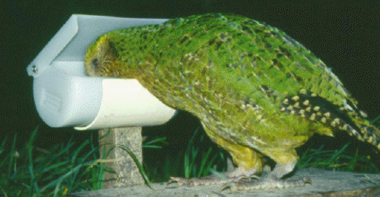High-ranking females tend to have daughters, whereas low-ranking females produce sons.  Recently, the management of the endangered kakapo in New Zealand ran into a sex ratio snag.  Supplemental feeding led to a hugely male-biased sex ratio.  Only once the managers talked to evolutionary biologists about influences on sex ratio, were they able to change the management so that females were also produced (Clout et al., 2002).

A kakapo (flightless nocturnal parrot!) using supplemental feed in New Zealand.  An unforeseen consequence of the feeding was that the sex ratio became highly male-biased.  Once managers realized the evolutionary link between maternal condition and the sex ratio, they were able to solve the problem. How? Simply by waiting to provide supplemental feed until after the females laid their eggs. 

Seasonal patterns.
Daan et al. (1996) argued that sex ratio may be skewed toward the sex that gets the biggest advantage from early age of first breeding. Early breeding species such as European kestrels (Falco tinnunculus) favor male-biased clutches early in the season. Males that get off to an early start have an advantage in securing mates (e.g., they can breed as yearlings). Larger, later-breeding species such as marsh harriers (Circus aeruginosus) favor female-biased sex ratio in early clutches, because in those species females may have a chance of moving up their age of first breeding.

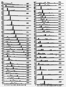
Changes in natality can cause waves in age structure. Mortality changes much less likely to caused pronounced spikes for two reasons:

1)  Births spiking in a single year also affect just one age class -- the cohort of new recruits. Mortality increases or decreases on the other hand will tend to affect several different age-classes.

2)  Some species have huge maximum fertilities that rarely result in successful recruitment. If conditions are right, however, there may be a huge pulse of reproduction in one season followed by years of minimal recruitment. Such favorable conditions might include plankton blooms (in marine systems) and fires (for trees). Species with very low birth rates (e.g., whales) are less likely to show such effects.

Strong cohort effects are sometimes seen in some marine fishes and plants (e.g., seedling recruitment of certain tree species following a forest fire).

Fig. 10.1. Diagram of a wave in the age structure of Norwegian herring, caused by a spike in natality (the numbers and letters are illegible, but you should still be able to get the idea). The X-axes show the age-classes, the Y-axes show the percentage of the total population represented by a given age-class. Each diagram represents a different year (1907 to 1958). Note that a strong pulse of large bars moves down and to the right as the very large cohort of recruits produced in 1908 moves through the population until they disappear in 1923 (about 2/3 of the way down the left column). Several sequential "waves" are visible in the sequence. Note also that for some time periods (e.g., 1947 to 1954, below middle of right-hand panel) the waves are much less distinct. The waves arise because only a few years are favorable for high spawning success and because the large clutch size of herring makes possible a very large maximal fertility.  Similar sorts of waves of massive recruitment can occur in plant species following forest fires. Huge areas will have stands of same-aged trees. 

References:

Clout, M.N., G.P. Elliott, and B.C. Robertson.2002. Effects of supplementary feeding on the offspring sex ratio of kakapo: a dilemma for the conservation of a polygynous parrot. Biological Conservation 107: 13–18

Daan, S., C. Dijkstra, and F.J. Weissing. 1996. An evolutionary explanation for seasonal trends in avian sex ratios. Behav. Ecol. 7: 426-430.

Kruuk, L.E.B., T.H. Clutton-Brock, S.D. Albon, J.M. Pemberton, and F.E. Guiness. 1999. Population density affects sex ratio variation in red deer. Nature 399: 459-461.

§§§§§§§§§§§§§§§§§§§§§§§§§§§§§§§§§§§§§§§§§§§§§§§§§§§§§§§§§§§§§§§

Return to top of page                        Go forward to notes for Lecture 11,  8-Feb