Lecture notes for ZOO 4400/5400 Population Ecology
Return to Main Index page
Go to Lecture 6 (where patterns of dispersion is mentioned as a population characteristic)
Go to Lecture 14 (lognormal distribution of ending sizes for stochastically varying population matrix projections)
Download Excel spreadsheet to generate the "expected" distribution for HW2
Dispersion
(for Homework # 2 and with reference to Lecture 6 -- population characteristics).
Homework: The first part of the homework deals with analyzing patterns of dispersion. Let me give a little background.
First, remember that the three primary patterns that concern us are clumped, random, and uniform.
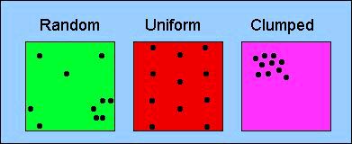
Fig. 6.3 from Lecture 6. Patterns of dispersion for organisms in a study area. By dividing the area into (invisible) quadrats, and counting the number of organisms per quadrat, we can assess the mean and variance of the number of organisms per quadrat, and thereby have a quantitative basis for deciding whether the observed dispersion is best described as random, uniform or clumped. Not that a random distribution will tend to have some clumps (as in the lower right) as well as very sparsely occupied areas (as in the upper right).
What can
we say about these patterns in a quantitative way?
Start with the expectation under a random
distribution. Consider that we divide our study area up into subplots.
Say we have 25 animals in a 10X10 plot (100 quadrats). What's the mean
number of animals per quadrat? Just the number of animals divided by the
number of quadrats. So, for this example, the mean occurrence or density
is 0.25 (animals per quadrat). When we really get out there, we will have
quadrats with no animals, some with one, some with two, and on up. What's
the probability distribution of number of animals per quadrat? Any problem
like this can be fitted to the discrete Poisson distribution.
Given a mean (our case is 0.25) it tells us the expected number of
"hits" per trial, if the "hits" are randomly distributed (in our case, number of animals per quadrat -- the original
example was the number of soldiers killed by horse kicks per
Prussian army battalion -- Simon Poisson, 1781-1840, was a French mathematician
and physicist).
{What continuous distribution should be very familiar to you from introductory statistics?}
The Poisson distribution has an interesting and memorable
property -- its mean equals its variance.
Given the mean number of "hits" we can generate the probability density
function (PDF) of the distribution. For our case, the mean number
of animals per quadrat is 0.25 (25 animals in 100 quadrats). We therefore
already have a prediction -- the variance of number of animals per quadrat
should also be 0.25, IF the dispersion
is random. Now we have a first criterion for assessing patterns of dispersion. But, it's just possible that we could construct a distribution
that had a mean equal to the variance that was still not random. We can
use a second histogram-based criterion to make our assessment. By using the probability density function (PDF)
we can generate an expected number of quadrats with 0, 1, 2, 3, 4, animals
respectively. I've done that for the 25 animal/100 quadrat case and the
expected distribution is
{78, 19, 2}
{ 0, 1, 2}
where the upper bracket is number of quadrats corresponding
to the number of animals found in them in the lower bracket. That is, we
expect 78 quadrats to contain zero animals, 19 to contain one, and 2 to
contain two. So even if we got a distribution with mean and variance =
0.25 if the values weren't reasonably close to 78 zeros, 19 ones and 2
twos, we'd have reason to believe that our animals weren't randomly distributed
across the landscape.
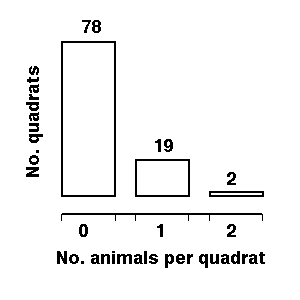
Fig. 1. Histogram of the discrete Poisson distribution with mean 0.25 for 25 animals distributed in 100 quadrats.
Note that the total "expected" is 23 (19*1 + 2*2 = 23). This occurs because the expectations are non-integer
but animals come in units. The "discreteness" comes from the number per quadrat (0, 1, 2, 3....) not from my
rounding the expectations (78, 19, 2) to integers. This kind of discrepancy will diminish as our study area (therefore number of animals per quadrat) increases -- another example of why larger sample sizes are almost always better.
Note that the shape of the distribution (unlike, say, the normal distribution) varies as the numerical
value of the mean varies. With a mean < 1.0 the
Poisson will have the hump (greatest number of quadrats expected with a
given number of animals) at 0 then 1 and on down. If the mean is > 1 though,
the distribution will look different. For a mean of 1.9 animals/quadrat,
for example, it will have the following expected values in 100 quadrats.
{15, 28, 27, 17, 8, 3, 1}
{ 0, 1, 2,
3, 4, 5, 6}
4.3 leads to {1, 6, 13, 18, 19, 17, 12, 7, 4, 2, 1} and its histogram is shown below:
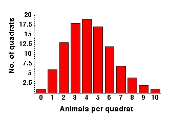
Fig. 2. Histogram of frequency distribution of number of animals per quadrat under a Poisson (random) expectation with a mean of 4.3 animals per quadrat (variance is therefore also 4.3). Note that the shape is different from other Poissons with different means. For a more uniform distribution, we would have more values near the mean (more 4s and 5s) and fewer farther from the mean (fewer zeros and fewer high numbers).
Deviations from the random (Poisson) expectation:
A uniform distribution with a mean of 4.3 would tend to have lots of values close to the mean (4s and 5s), leading to a low variance. It would also have a deficiency of zeros (not much open space).
A clumped distribution with this mean would have lots of zeros and more quadrats with high numbers of animals (that is there would be few quadrats with 4s and 5s, the values close to the mean). Those far-from-the-mean values would drive up the variance, leading to a high variance.
Note also that anything beyond the last value given
will round to 0. There is a small probability of having 5 individuals
in our observed vector of animals/quadrat (approximately a one in 10,000),
but that expectation rounds down to 0 because I am using integer math.
(reasonable, given that we are talking about unitary animals or plants
here).
How a large variance arises. One more
thing. What kinds of values can throw the variance away from the "expected"?
For our cases with mean 0.25 any values out at high numbers per cell will
greatly inflate the variance. Remember that the variance is calculated
as a squared deviation from the mean. Changes in the 0 and 1 cells will
be squaring values of approximately one, so they will add approximately
one unit per missing or extra quadrat to the variance. But every instance
of a value three or four from the mean will add none or sixteen units to
the variance sum. In any actual implementation of an analysis of dispersion,
that means that a few herds or flocks out there could quickly move us
away from a reasonable fit to the hypothesis that the animals are randomly
distributed by our mean variance equivalence criterion. In the case of a higher mean (say the 4.3 example) quadrats containing zero animals will also be far from the mean and will inflate the variance.
Questions to ponder: Consider extreme cases: what is the absolute
maximum clumped pattern? How many zeros, ones, twos do we expect
then? Where will the excesses and deficiencies be relative to the
Poisson distribution? How about the most uniform distribution possible?
What happens to the variance in each of those two extreme cases?
Summary:
"Baseline" or "null" model is the random expectation modeled by the Poisson distribution.
That produces 2 criteria for assessment.
The first is the relationship of the mean to the variance.
The second is the distribution of quadrat numbers in the histogram (as in Figures 1 and 2). [You should also try to learn to "visualize" the histogram given only the bracketed double-list format].
Clumped:
1)
If mean < variance observed distribution is tending toward clumped
2)
Many quadrats will have values far from the mean; a histogram with very long tails, possibly even U-shaped (many values at zero, some at a high value and none in the middle)
Random:
1) If mean = variance, observed distribution matches the distribution expected under the Poisson probability density function (PDF)
2)
Peak of frequency distribution will be near the mean, but the histogram can have fairly long tails
Uniform:
1)
If mean > variance observed distribution is tending toward uniform
2)
Most quadrats will have values close to the mean; a histogram heavily peaked near the mean, with few values in the tails of the distribution
_______________________________________________________________________________________________________________________
§§§§
§§§§§§§§§§§
§§§§§§§§§§§§§
§§§§§§§§§§§§§§
§§§§§§§§§§§§§
§§§§§§§§
Return to top of page