Lecture 18 (27-Feb-13) Discrete logistic chaos (continued) --
    divergence from (nearly) identical starting points;
    experimentally induced chaotic population fluctuations

Return to Main Index page                          Go to movie of discrete logistic 2-cycle (r = 2.2) case      

  Go to movie of discrete logistic chaos (r = 3) case           Go to movie of discrete logistic converge-to-K (r = 1.5) case

Go to back to lecture 17, 25-Feb              Go forward to lecture 19 of 1-Mar

Last time I introduced the discrete logistic model and showed how it can generate undamped oscillations and chaos.

Let's look at another interesting aspect of the behavior of the discrete logistic with high values of r (> 2.692) in the chaos region. Our 1-dimensional map with N(t) vs. N(t+1) actually provides an illusion of order. If we know the population size at t it is easy to predict the size at t+1 (that is the points lie along a well-defined continuous smooth curve, as shown in the graph below).

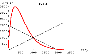
Fig. 18.1. Plot of N(t) vs. N(t+1) for the discrete logistic with r = 3.5 (chaotic region) and K = 1000. Note that for any given value of N(t) it is easy to predict the value of N(t+1). The points all fall along the smooth red curve, but try the box-step method of tracing the map and see how wild the trajectory becomes. Main point: for a single time step in the future, knowing an approximate value for our current state (population size) tells us pretty closely where we'll be.

Tips on reading the maps. 
1) The 1:1 positive-slope line.  This line helps us read the map. We can determine sequential population size numbers by bouncing back and forth from the curve to this line. 
2) The negative-slope 45° line.  This line helps us decide whether the dynamics will settle on a single stable equilibrium (when the line crosses only at the intersection of the two straight lines) or whether population size will oscillate (2, 4, or higher number of oscillation sizes) or be chaotic.  Oscillations or chaos will be the outcome when the curve crosses the negative-slope line more than once.  The steeper the curve, the more likely it is that it will approach the realm of chaos. 
3) The curve. This is what we use to predict the population size one time step in the future. Remember that this is a deterministic system. If we know exactly where we are, we can predict exactly where we will be on the next time step. The one-step map yields a smooth curve. As we go to a map with a larger number of time steps (as below, in Fig. 18.2), the curve atomizes into a random-looking set of points. The scatter arises because even two starting points very close together will diverge more and more over time, so that 10 or 20 time steps later, two nearly identical starting points will have very different destinations.  But ... if we start at a given (exact) point, and run the equations over and over, we will always go to the same destination. 
4) The axes.  We are plotting population size against itself (at some later time), which is why these are called one-dimensional maps. 

Let's contrast that orderliness and predictability with what we find if we take larger time steps, as in the graph below. Whereas it was easy to predict N(t+1) from N(t), the plot of N(t+15) against N(t) is all over the place -- chaos.  Points that started close together at time t, can be very far apart at time t+15. 

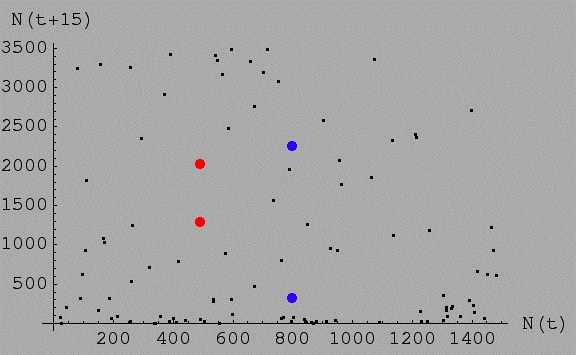
Fig. 18.2. Plot of N(t) vs. N(t+15) for the discrete logistic with the same values as in Fig. 18.1 -- r = 3.5 (chaotic region) and K = 1000.
Note that for any given value of N(t) it is possible to wind up with almost any value of N 15 time steps later. For example, the red dots represent two populations that started at sizes of 500 and 501. That is, they started at almost exactly the same size (their position along the X-axis, which is why they line up well vertically). 15 time steps later one is at N = 1,296, the other is at N = 2,030.
The two blue dots started at 799 and 800 respectively -- 15 time steps later one is down at 321, the other is up at 2,252.
What about all the black dots? They represent a very disorderly (in fact chaotic) smattering of relationships between N(t), the X-axis value,
and N(t+15), the Y-axis value. For any particular value along the X-axis, we can wind up almost anywhere else 15 time steps later.
[Check this out by noting that dots at the same place on the X-axis can be at very different spots on the Y-axis, just as we saw for the two different red dots]. Where you start tells you very little about where you will be only a short time (15 time steps) later. Put differently, the outcome is extremely sensitive to the initial conditions. Any particular initial condition has a deterministic outcome. If we start at exactly N(t) = 296. 0341 and plug that into the discrete logistic of Eqn 18.1, we will always go to exactly the same value at time t +15 (because the system is deterministic, as opposed to stochastic). But that trajectory will tell us almost nothing about where we are likely to end up if we start at N(t) = 296.0342 and run the sequence for any extended period of time (they start close together and lose any similarity as time progresses).

Main point: Knowing the approximate value of the current state tells us almost nothing about the state of the system in the more distant future. Even if we start at two different points that are only very slightly different, the trajectories diverge widely over time -- this is one of the defining characteristics of chaotic dynamics.

Under chaos, an infinitesimally small change in initial conditions leads to dramatic changes in long term trajectories. Chaos produces a discontinuous response to a continuous change in input (arbitrarily small changes in input produce radically different endpoints),

How long does it take for chaos to get going if little r is changing? If r fluctuates, how long till we see chaotic fluctuations? That may be very hard to tease apart. Changes in r can cause the population size to fluctuate. Usually, though, we'd see cycles or very large amplitude fluctuations within a few birth pulses (breeding seasons).

Go back and look at how we defined the composition of little r very early in the course.

Question to ponder: what are some differences and similarities between populations subject to environmental stochasticity (Lecture 16) and populations subject to deterministic chaos (Lectures 17& 18)?

Let's contrast the unpredictability of N with a high r, with the predictability of N with low values of r. 

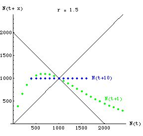
Fig. 18.3. One-dimensional map of N(t) against N(t+x) showing complete predictability of N at time 10 when r is low. The green (curved-line) dots show N(t+1) for various values of N.  By time t+10, all starting values will converge on the carrying capacity.  The blue dots therefore fall along a straight line of Y = 1,000 that goes through the two straight black lines (which have slopes +1 and -1). 

Question to ponder: with r in the 2-cycle range, what would the map of N(t+10) against N(t) look like? 
[ Look back at Fig. 17.5 if you don't come up with an answer right away]. 

Experimentally induced chaos. The experimental work of Costantino et al. (1997) shows that chaotic fluctuations can occur (at least under special circumstances) -- whether chaotic fluctuations regularly occur in natural populations is still an open question. By the way, the r value necessary to generate chaotic dynamics is 2.692 or greater. That corresponds (l = e^r) to a l of 14.8! Now that's rapid growth! Only invertebrates or possibly certain fish populations are likely to have those kinds of possible growth rates.

How would we demonstrate chaotic population dynamics experimentally? Costantino et al. (1997) claimed to have induced chaotic population dynamics experimentally in Tribolium flour beetles.

Tribolium, a pest of stored grains.  It has a very high r, which was forced even higher by the experimental conditions used by Costatino et al. 

What evidence would we like to see in order to be confident that their claims are valid? Fluctuations that lack apparent pattern (irregular increases and decreases in population size over time) are certainly insufficient evidence. Many populations fluctuate, some might even fluctuate wildly, without the fluctuations being due to chaotic dynamics (meaning a specific mathematical outcome of, for example, pushing a simple deterministic discrete logistic to chaos by increasing r). One of the strongest pieces of evidence would be the progression of patterns as we push the parameters (such as r). Eqn 18.1 (the discrete logistic) responds to increased r by moving from

highly stabilizing convergence toward a single equilibrium point (K) at r-values > 2.0,
to undamped 2-cycle oscillations (r between 2.0 and 2.562),
to 4-cycle oscillations,
to 8-cycle
and
    then
        cascades quickly to c_ha^o Ti c dynamics above a threshold value of r > 2.692.

If the experimental population moves through cycles of increasing cycle size as we increase r, our confidence increases greatly in hypothesizing deterministic chaos as the underlying force for wild population fluctuations.

Go to movie of discrete logistic 2-cycle (r = 2.2) case        Go to movie of discrete logistic chaos (r = 3) case

Go to movie of discrete logistic converge-to-K (r = 1.5) case

Other uses of chaos theory (not for testing, just general interest):

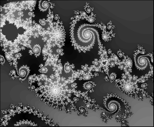
A representation of a small portion of the Mandelbrot set (a fractal image produced by a deterministic chaos algorithm).   Notice the repeated motifs.  Each of the swirls contains within it a series of similar swirls. Many more such images are available by Googling for "fractal images" or "Mandelbrot set". 

The intricate patterns of branching in root hairs and tree branches also seem to represent fractal (chaotic) processes. 

The dynamics of weather may also, often, be driven by deterministic processes with high forcing values.  That's one of the reasons the weather can be so hard to predict.  If we had exactly the right equation (not the discrete logistic, but one with similar properties) and if we knew exactly what the initial conditions were, we should be able to predict the weather exactly.  Even the slightest misestimation of the current conditions, however, will lead to increasingly large deviations between our estimated weather trajectory and the actual trajectory driven by the deterministic (but chaotic) process. 

References:

    Costantino, R.F., Desharnais, R.A., Cushing, J.M., and Dennis, B. 1997. Chaotic dynamics in an insect population. Science 275: 389-391.

§§§§§§§§§§§§§§§§§§§§§§§§§§§§§§§§§§§§§§§§§§§§§§§§§§§§§§§§§§§§§§§

Return to top of page                   Go forward to Lecture 19 of 27-Feb